A Reduced Transport Model for Ion Heat Diffusivity by Gyro-Kinetic Analysis with Kinetic Electrons in Helical Plasmas

(1)

A Reduced Transport Model for Ion Heat Di

ﬀ

usivity by

Gyro-Kinetic Analysis with Kinetic Electrons in Helical Plasmas

Shinichiro TODA, Motoki NAKATA, Masanori NUNAMI, Akihiro ISHIZAWA

1)

_,

Tomo-Hiko WATANABE

2)

_{and Hideo SUGAMA}

National Institute for Fusion Science, 322-6 Oroshi-cho, Toki, Gifu 509-5292, Japan

1)_{Graduate School of Energy Science, Kyoto University, Gokasho, Uji, Kyoto 611-0011, Japan} 2)_{Department of Physics, Nagoya University, Furo-cho, Nagoya, Aichi 464-8602, Japan}

(Received 14 April 2017/Accepted 27 July 2017)

A high ion temperature plasma in the Large Helical Device is examined in the case in which the ion temper-ature gradient mode is unstable. The nonlinear gyro-kinetic simulation is performed to evaluate the turbulent ion heat diﬀusivity with the kinetic electron response. It is clarified that the decay time of zonal flows [S. Ferrando-Margaletet al., Phys. Plasmas14, 122505 (2007)] decreases radially outward due to the trapped electron and the ion energy transport increases outward. To reduce the computational cost for applying to the dynamical transport simulation, an extended transport model for the ion heat diﬀusivity in terms of the mixing length estimate and the characteristic quantity for the linear response of zonal flows is proposed.

c

2017 The Japan Society of Plasma Science and Nuclear Fusion Research

Keywords: transport model, zonal flow, gyro-kinetic simulation, turbulence, helical plasma DOI: 10.1585/pfr.12.1303035

Turbulent transport is one of the most critical issues for plasma confinement in magnetic fusion devices. The-oretical expressions for the turbulent transport due to the various instabilities were reviewed [1]. Recently, a large number of the gyro-kinetic simulations which are applied to the turbulent transport have been performed in toroidal plasmas, e.g.[2–8]. The gyro-kinetic analysis results in tokamak [9–11] and helical [12–14] plasmas have been studied with the experimental observations. Gyro-kinetic simulations of helical plasmas require a large number of mesh points along the field line in order to capture the he-lical ripple structure. Therefore, the gyro-kinetic analysis in helical plasmas consumes the larger computer resources than for tokamaks. In helical plasmas, it is not practical to perform the nonlinear gyro-kinetic simulation at each time step of the dynamical transport code. The reduced model, which reproduces the nonlinear gyro-kinetic analysis re-sults, is needed for the dynamical transport simulation in helical plasmas.

The GKV code [15] has been used to examine the ion temperature gradient (ITG) mode and zonal flows in the Large Helical Device (LHD) for studying the turbulent transport [13]. The gyro-kinetic simulation with the adi-abatic electron is performed for the high ion temperature LHD discharge (shot number 88343 [16]). The ion energy flux by the ITG mode instability agrees with the experi-mental results [13, 14]. The reduced model for the ion heat diﬀusivity is proposed [14] by the simulation with the adi-abatic electron. This reduced model is the function of the

author’s e-mail: [email protected]

linear growth rate for the ITG mode and the zonal flow decay time [17, 18]. In tokamak plasmas, the gyro-kinetic analysis at each time step is globally performed in the dy-namical transport simulation [19, 20]. How to apply the reduced model of the turbulent ion heat diﬀusivity from the gyro-kinetic simulation with the adiabatic electron to the transport code has been shown in helical plasmas [21]. The simulation with the kinetic electron shows the larger ion energy flux than the experimental results in the high-Ti

LHD discharge [22]. On the other hand, the electron and ion energy fluxes of the simulation results with the kinetic electron are close to those of the experimental results in the low-Ti#88343 discharge [23]. The simulation result with

the adiabatic electron in this low-Tidischarge shows that

the ITG mode becomes stable aroundρ(=r/a)=0.5. The effect of the kinetic electron induces the enhancement of the linear growth rate of ITG modes [4,22]. To show the re-duced transport model for the turbulent ion heat diffusivity, the effect of the kinetic electron on the plasma instability should be included.

In this study, the reduced model of the ion heat diff u-sivity for the ITG mode is proposed by solving the gyro-kinetic equation in terms of the electron in addition to the ion to examine the effect of the kinetic electron. The same method with the gyro-kinetic analysis using the adiabatic electron [14] is adopted. The nonlinear gyro-kinetic simu-lation is performed to evaluate the ion heat diffusivity. The effect of the kinetic electron on the linear response of zonal flows is studied. The linear gyro-kinetic simulation is also performed for the reduced model in order to reproduce the

c

2017 The Japan Society of Plasma

(2)

Fig. 1 Time evolution of the ion energy flux.

value of the ion heat diﬀusivity by the nonlinear analysis. We examine the turbulence driven by the microin-stabilities in LHD plasmas, using the gyro-kinetic local flux tube code GKV [15]. Based on the temperatures ra-dial profiles, density rara-dial profiles, and field configuration from the LHD experimental results of the high-Ti phase

att = 2.233 s [16], the electron and ion temperature

gra-dients, R/LTe andR/LTi, the density gradient R/Ln, and

the safety factorqradially change. The GKV simulation with the kinetic electron is performed withR = 3.75 m.

The β(= 2μ0n(Te+Ti)/B2) value is 0.3% at ρ = 0.65.

To reduce computer resources and perform the nonlinear analysis in the wide plasma parameter region, we take the smaller number for the Fourier modes and the smaller number of the grid points in this simulation than in the case in [22]. The total Fourier mode numbers in the ˜kxand

˜

k_y directions are 9 and 6 in the regions−0.5 ≤ k˜x ≤ 0.5

and 0.0 ≤ k˜_y ≤ 0.5, where ˜kx(= kxρi) and ˜ky(= kyρi)

are the radial and poloidal wavenumbers. The nonlinear GKV simulations are carried out at ten radial points be-tweenρ = 0.46 andρ = 0.80. As an example, the time evolution of the ion energy fluxQiatρ = 0.65 is shown

in Fig. 1. The value of timetis normalized byR/vti. The

saturation of the ion energy flux is obtained in the nonlin-ear phase. The averaged value of the ion energy flux in the time interval 50< t < 100 is 0.12 MW/m2. In [22], the averaged value of the ion energy flux in the time interval 50<t<80 is about 0.13 MW/m2_{, when the Fourier mode} numbers in the ˜kxand ˜k_ydirections are 169 and 43. Even if

the number of the Fourier modes is small, the close value of the ion energy flux is obtained in this study. This is be-cause the peaks of the electrostatic potential fluctuation are found in the regions 0.0 ≤_k˜_x_,y_≤_{0.5 and the values of the} electrostatic potential fluctuation in the regions ˜kx_,y> 1.0

are extremely small. The averaged value of the ratio of the electromagnetic contribution Qem

i to the total ion energy

fluxQiin the time interval 50<t<100 is 0.33%, because

of the low beta 0.3% plasma. The finite beta eﬀect is neg-ligibly small to the ion electrostatic flux in this study. The values of ¯χiby the simulation with the kinetic electron are

from two to three times larger than those by the simulation

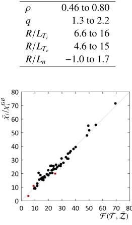
Table 1 Parameter region in the nonlinear simulations.

ρ 0.46 to 0.80

q 1.3 to 2.2

R/LTi 6.6 to 16

R/LTe 4.6 to 15

R/Ln −1.0 to 1.7

Fig. 2 Comparison of ¯χi/χGBi from the nonlinear gyro-kinetic

simulation with the model functionF( ¯T,Z¯). The cir-cles and the boxes show the results in high-Tiand low-Ti

phases.

with the adiabatic electron. The bar ¯ shows the averaged value in the time interval of the nonlinear saturation phase. The time evolutions of the squared turbulent potential fluc-tuation, T

= Σkx˜,˜k_y0

_φ_˜

˜

kx,˜k_y

2

/2and the squared zonal flow potential,Z

= Σk˜x _φ_˜

˜

kx,k˜y=0 2

/2

are studied, where ˜

φis the electrostatic potential fluctuation which is defined as ˜φ=φ/(Tiρi/(eR)). The bracketdenotes the averaged

values along the magnetic field line. The nonlinear satura-tion is seen in the time evolusatura-tion ofT andZ.

The normalized electron and ion temperature gradi-ents are artificially altered at 0.8 and 1.2 times the exper-imental values at ten radial points. This is because the ion energy flux decreases with the reduced gradient by 20% and close to the experimental value [22]. The pa-rameter range in which the nonlinear simulation has been performed is shown in Table 1. The transport coeﬃcients

¯

χi/χGBi by the nonlinear simulation are compared with a

model function of ¯T and ¯Zby the circles in Fig. 2. A fit-ting function for the ion heat diﬀusivity is defined by

¯ χi

χGB i

=F( ¯T,Z¯)≡ C1T¯

α

C2+Z¯ 1 2/T¯

, (1)

withα=0.46,C1=5.5×10−2, andC2=2.2×10−2, where χGB

i is the gyro-Bohm diﬀusivity. The relative error for

fit-ting ¯χi/χGBi byF is 0.12, where the relative error is defined

as the root mean square of( ¯χi/χGBi )/F −1

(3)

C2in this article are similar to those of the coeﬃcients by the simulation with the adiabatic electron [14]. In [23], the gyro-kinetic simulation is performed in the low-Ti phase

for #88343 in the LHD. The values of the normalized ion heat diﬀusivity by the model (1) are comparable with the values by the nonlinear simulation at three radial points in the low-Tiphase [23] with the boxes in Fig. 2.

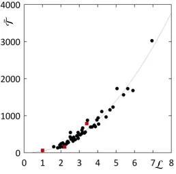
To represent the contributions of the turbulent fluctu-ations and zonal flow fluctufluctu-ations to the turbulence level by the linear gyro-kinetic analysis, the simulation is per-formed with the kinetic electron. The values of the lin-ear growth rate by the simulation with the kinetic electron are several times larger than those by the simulation with the adiabatic electron. The instabilities are driven by the ITG mode because the real frequency is negative and the mode rotates towards the ion diamagnetic direction. Fig-ure 3 shows the relation between the turbulence fluctuation

¯

T and the mixing length estimateL ≡( ˜γk˜_y/k˜2_y)dk˜y

[24] integrated over 0.1 ≤ _k˜_y _≤ _{0.5 with the circles, where} ˜

γk˜y(=γ˜ky/(vti/R)) is the linear growth rate. The turbulence

fluctuation ¯T is approximated by ¯

T =CTLa, (2)

with the coeﬃcientsCT = 4.8×10 and a = 2.1. The

three values of ¯T by the nonlinear simulation in the

low-Tiphase are found to be comparable with those by Eq. (2)

with the boxes in Fig. 3. The turbulent transport level is not only determined by the mixing length estimate. The level of the turbulence is also determined by the interac-tion between the turbulence and the zonal flows shown in Eq. (1). The linear zonal flow response function is defined by Rk˜x(t) ≡

˜ φk˜x,˜ky=0(t)

/_φ˜_˜_k

x,˜ky=0(t=0)

. We examine the linear zonal flow response using the field configuration for the high-Tiand low-Tiphases in the LHD #88343

dis-charge. In the low-Tiphase, the magnetic field

configura-tion is shifted inward and the major radius is close to 3.6 m. In the inward shifted field configuration, the helical mag-netic structure can enhance the generation of zonal flows [25]. The linear zonal flow response depends on the

mag-Fig. 3 Comparison of the time-averaged turbulent fluctuation ¯T with the mixing length estimate,L. The circles and the boxes represent the results in high-Tiand low-Tiphases.

netic field configuration but does not depend on the plasma profile. Note that we set the value of ˜kxaround 0.25,

be-cause there is a peak of the wavenumber spectra around ˜

kx=0.25 as the results of the nonlinear simulation. To

ex-amine the correlation betweenR˜kx(t) and the fluctuation of

zonal flows ¯Z, the zonal flow decay time [18] is employed. The zonal flow decay time is defined byτZF≡

_τf

0 dtRkx˜ (t),

whereτf is the upper limit oftin the integral. Here, we set

τf =15R/vti, because the zonal flow decay time does not

change significantly forτf >15R/vti. The correlation time

of the turbulence in the nonlinear simulation result shown in Fig. 1 is shorter than 15R/vti, thusR˜kx(t) forτf >15R/vti

does not influence the excited zonal flow level. The zonal flow fluctuation ¯Zis approximated by the linear simula-tion results as the funcsimula-tion of ˜τZF(=τZF/(R/vti)) and ¯T,

¯

Z=Czτ˜bZFT¯ c_,

(3) withCz=0.0061,b=1.6 andc=1.4. The comparison of

¯

Zwith 0.0061˜τ1.6

ZFT¯

1.4_{is shown in Fig. 4. The circles and} boxes represent the simulation results in the high-Ti and

low-Tiphases.

We study the diﬀerence of the linear zonal flow re-sponse with the kinetic electron from that with the adia-batic electron. Figure 5 represents the time trace of the

lin-Fig. 4 The plots for the comparison of ¯Zwith 0.0061˜τ1.6

ZFT¯

1.4_.

The circles show the simulation results in the high-Ti

phase and the boxes represent those in the low-Tiphase.

Fig. 5 Time trace of Rk˜x=0.25(t) as the results with the

(4)

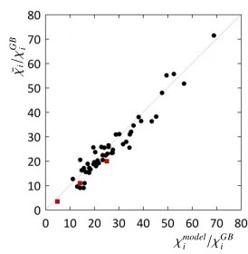
Fig. 6 The comparison of the nonlinear simulation results with the kinetic electron, ¯χi with the model predictions of

Eq. (4),χmodel

i . The circles and the boxes show the results

in high-Tiand low-Tiphases.

ear zonal flow response functionRkx˜ (t) for the simulation results with the adiabatic electron (the solid curve) and the kinetic electron (the dashed curve) atρ = 0.80. The lin-ear zonal flow response function with the kinetic electron decays faster than that with the adiabatic electron. The zonal flow decay time decreases radially outward due to the trapped electron [17]. The turbulence fluctuation ¯T in-creases outward. Therefore, the ion energy flux is found to increase radially outward in this study and in [23]. In the adiabatic electron case, the zonal flow decay time in-creases outward and the ion energy transport dein-creases out-ward [14].

When we substitute Eqs. (2) and (3) into Eq. (1), the reduced model which represents the ion heat diﬀusivity in terms of the linear plasma parameters by the simulation with the kinetic electron is shown as

χmodel i

χGB i

= A1LB1

A2+τ˜BZF2/LB3

, (4)

where the coeﬃcients are given by A1 =

C1CTα+1−c/2C

−1/2

z =1.3×101 andA2 =C2CT1−c/2C

−1/2

z =

0.90. The exponents are also given byB1 = αa = 0.97,

B2 = b/2 = 0.80, and B3 = a(1 −c/2) = 0.63. By the linear gyro-kinetic simulation, the value of χmodel_i is obtained. The ion heat diﬀusivities χmodel_i and ¯χi are

compared with the circles in Fig. 6. The reduced model reproduces the nonlinear simulation results ¯χi for the

relative error 0.16. The values of the ion heat diﬀusivity by the reduced model (4) are comparable with those by the nonlinear simulation at three radial points in the low-Ti

phase [23] with the boxes in Fig. 6.

In summary, the gyro-kinetic simulation with the ki-netic electron is performed to show the reduced transport model for the turbulent ion heat diﬀusivity. At first, the ion heat diﬀusivity is evaluated from the nonlinear simula-tion for high-Tiplasma in the LHD, where the ITG mode

is destabilized. To investigate the wide plasma parameter region, the smaller number of Fourier modes is taken than

the case in [22]. The model function for the ion heat diﬀ u-sivity is shown in terms of ¯Tand ¯Z. Next, the terms ¯T and

¯

Zin the model function are approximated by the terms of the mixing length estimate and the zonal flow decay time evaluated from the linear simulation. The use of the lin-ear simulation results enables us to reproduce the nonlin-ear simulation results by the reduced model. The decay of zonal flows with the kinetic electron becomes faster. The decay time of zonal flows is found to decrease radially out-ward and the ion energy transport increases outout-ward due to the trapped electron. The dependence of the reduced model for the turbulent diﬀusivity on the field configuration (e.g., for low-Tiphase) and the plasma profiles for the LHD and

different devices has been investigated. The model func-tions for the turbulent heat and particle diffusivities were shown in the tokamak plasmas [26]. In this study, the time averaged value in the nonlinear saturation phase of the ratio of the electromagnetic contribution to the total electron en-ergy flux becomes about 30%, despite the low beta plasma. If the larger number of the modes is taken, the electromag-netic energy flux becomes smaller in the total electron en-ergy flux [22]. The reduced transport models for the elec-tron heat diffusivity and the particle diffusivity in addition to ion heat diffusivity will be studied.

This work was partly supported by JSPS KAK-ENHI Grant Numbers 23561002, 16K06941, and 17K14899, the NIFS Collaboration Research programs, NIFS16KNST093, NIFS16KNTT035, and the Collabora-tive Research Program of Research Institute for Applied Mechanics, Kyushu University, 28FP-1.

[1] J.W. Connor and H.R. Wilson, Plasma Phys. Control. Fu-sion36, 719 (1994).

[2] X. Garbetet al., Nucl. Fusion50, 0433002 (2010). [3] F. Jenko and W. Dorland, Plasma Phys. Control. Fusion43,

A141 (2001).

[4] J. Candy and R.E. Waltz, J. Comput. Phys.186, 545 (2003). [5] T.-H. Watanabe, H. Sugama and S. Ferrando-Margalet,

Nucl. Fusion47, 1383 (2007).

[6] P. Xanthopouloset al., Phys. Rev. Lett.99, 035002 (2007). [7] M. Nunamiet al., Plasma Fusion Res.6, 1403001 (2011). [8] A. Ishizawaet al., Phys. Plasmas21, 055905 (2014). [9] M. Kotschenreutheret al., Phys. Plasmas2, 2381 (1995). [10] C. Hollandet al., Phys. Plasmas18, 056113 (2011). [11] T.L. Rhodeset al., Nucl. Fusion51, 063022 (2011). [12] H.E. Mynick, N. Pomphrey and P. Xanthopoulous, Phys.

Rev. Lett.105, 0950094 (2010).

[13] M. Nunamiet al., Phys. Plasmas19, 042504 (2012). [14] M. Nunami, T.-H. Watanabe and H. Sugama, Phys. Plasmas

20, 092307 (2013).

[15] T.-H. Watanabe and H. Sugama, Nucl. Fusion 46, 24 (2006).

[16] K. Tanakaet al., Plasma Fusion Res.5, S2053 (2010). [17] H. Sugama and T.-H. Watanabe, Phys. Plasmas13, 012501

(2006).

[18] S. Ferrando-Margalet, H. Sugama and T.-H. Watanabe, Phys. Plasmas14, 122505 (2007).

(5)

[21] S. Todaet al., J. Phys.: Conf. Ser.561, 012020 (2014). [22] A. Ishizawaet al., Nucl. Fusion55, 043024 (2015). [23] A. Ishizawaet al., Nucl. Fusion57, 066010 (2017). [24] J. Wesson, Tokamaks, 2nd ed. (Oxford University Press,

1997) p.198.

[25] T.-H. Watanabe, H. Sugama and S. Ferrando-Margalet, Phys. Rev. Lett.100, 195002 (2008).