and Asymmetric Response to Past
Shocks in the Malaysian Bond Market
**Maya Puspa Rahman*, Mohd Azmi Omar andSalina H. Kassim
ABSTRACT
The exercise of modelling the risk and volatility of corporate bonds is undertaken through credit spreads analysis, a practice normally used in bond pricing and risk management. Despite the rapid growth of the Malaysian bond market, very few studies on the behaviour of credit spreads, and whether its volatility is influenced by external shocks have been conducted. This paper aims to unveil the trends and behaviour of credit spreads during the 2007/2008 global financial crisis. It examines the credit spreads of the Malaysian bond market by modelling the conditional variance and asymmetric response to past shocks of the long and short term investment and non-investment grade papers. A generalised autoregressive conditional heteroscedasticity (GARCH) is applied to 10 different ratings and maturity over the period ranging from 1 August 2005 to 31 December 2011. More specifically, modelling the asymmetry via the threshold GARCH (TARCH) and exponential GARCH (EGARCH) models meets the aim of this paper which examines the asymmetric response to past shocks of the Malaysian bond market during the 2007/2008 global financial crisis. The empirical analysis of this paper provides evidence of strong time-varying conditional variance of the Malaysian bond credit spreads with
* Corresponding author: Maya Puspa Rahman is an Assistant Professor at the Department
of Economics, Kulliyyah of Economics and Management Sciences, International Islamic University Malaysia, Kuala Lumpur, Malaysia. Email: [email protected].
Mohd Azmi Omar is a Director General of Islamic Research Training Institute (IRTI), Jeddah, Kingdom of Saudi Arabia
Salina H. Kassim is an Associate Professor at the Department of Economics, Kulliyyah of Economics and Management Sciences, International Islamic University Malaysia, Kuala Lumpur, Malaysia.
the expectation of future rate being the main determinant for credit spreads. Additionally, the evidence also indicates that past news or shocks as well as forecast variance are important in explaining the volatility of the spreads. The insignificant TARCH and EGARCH coefficients, nonetheless, indicate that there is no evidence of asymmetric response to past shocks in the volatility of bond spreads.
Keywords: Credit Spreads Analysis, EGARCH, GARCH, Malaysian Bond Market, TARCH, Volatility
JEL Classification: C58, G01, G12
1. Introduction
Bond investment plays a critical role in the development of the capital
market in any country. In Malaysia, the size of the total outstanding
bond stood at USD315 billion, making it the third largest bond market in Asia after Japan and Korea.1 Domestically, the Malaysian bond market had grown by more than 400 per cent since the year 2000, from the amount outstanding of RM225 billion to RM1058 billion as at June
2014 (Securities Commission, 2014). In order to make a well-informed decision on bond investments, it is important to understand the true nature of credit risk as it allows investors to take advantage of new opportunities, compare relative risks and returns between different bonds, maximise yields and diversify investment risk. Hence, a timely and adequate information on credit risks of bonds is crucial.
The traditional approach of assessing credit risk based on a ‘straight
ratios’ analysis is deemed to be inefficient and backward looking.
This is because it is unable to meet the current urgent needs of fast decision making and informed decisions. Hibbert, Pavlova, Barber, and Dandapani (2011) highlight this issue and agree that credit spreads
analysis is inherently forward looking and reflects the expectation of
default or credit risk. Credit risk analysis was initially highlighted by
Merton (1974) and is reflected by what is termed as credit spreads2 (Avramov, Jostova, & Philipov, 2007; Berman, 2005; Elton, Gruber, Agrawal, & Mann, 2001; Hibbert et al., 2011). Theoretically, credit
spreads reflects the compensation given to investors for bearing higher
risks in holding corporate bonds (credit risk), and is believed to be an
1 Size of local bond market as at December 2014 and is compared to a group of seven Asian
countries namely, Japan, Korea, Malaysia, Thailand, Singapore, Indonesia and Philippines (ADB, 2015).
appropriate tool to analyse the risk-return trade-off in the corporate bond market. Other than that, according to the classical work of Merton
(1974), spreads also provides an early signal to a firm’s probability of default when its value falls below the amount that the firm owes.
Mathematically, spreads is calculated by taking the difference between the yield of a corporate bond (risky asset) and government bond (risk-free asset) of similar maturity which is often used to price the credit risk of the new issuance of corporate bonds (Fabozzi, 2000).
Apart from possessing a critical role in bond pricing, credit spreads
also reflects investors’ behaviour as it changes systematically with
changes in the economy. For example, during an economic downturn, lesser demands for corporate bonds lead to a downward pressure on its price hence, pushing its yield to be relatively higher to government bonds, thereby resulting in the widening of the spreads (Demchuk & Gibson, 2006; Fabozzi, 2007; Krainer, 2004). This is evident during
the 2007/2008 global financial crisis where the daily spreads of the
Malaysian 10-year AAA and 10-year Malaysian Government Securities
(MGS) from the year 2005 to 2011 shows a significant spike in the middle of 2008 (Figure 1). This pattern suggests that credit risk significantly increases during the crisis. It was only by the year 2009 that credit
spreads shows a decreasing pattern, thereby indicating a recovery in the local bond market and a rejuvenated local economy (RAM Rating Services Berhad, 2010).3 A comparison of the situation then with the leading US bond market indicates that the spreads of the 10-year AAA US industrial corporate bond and the 10-year US Treasury bonds had also widened by 189.2 basis points around November 2008, the highest spreads since 2006 (Figure 2).
As credit plays an important role in the pricing of corporate bonds
and the reflection of investors’ behaviour during the different states
of the economy, many studies have explored the behaviour of credit spreads as well as those factors determining its changes. Some studies such as Batten, Fetherston, and Hoontrakul (2006), Batten and Hogan (2003) and Manzoni (2002) provide interesting empirical evidence to show the persistence of volatility clustering of the changes in spreads.
In financial econometrics, the presence of volatility clustering is termed
as heteroscedasticity and this signals that the variance of the error term is not constant but that it varies over time. This variance contains additional information of the behaviour of the dependent variable, hence, is essential to be modelled (Engle, 2001).
3 Rahman, Omar, and Kassim (2013) provide the latest discussion on the trend of spreads
0.0 50.0 100.0 150.0 200.0 250.0 300.0
Mar-11 Nov-08 Aug-06
SPREAD
Figure 2: Credit Spreads of 10 year US Treasury and 10 year AAA US Industrial Corporate Bond
Source: Bloomberg Corporate Spread Matrix, Rahman et.al (2012).
Ample research have been undertaken to look at credit spreads which focuses on developed bond markets such as those in the US, United Kingdom and Japan.4 Despite the rapid growth and significance of the Malaysian bond market in developing the Malaysian economy, Figure 1: Credit Spreads of Malaysian 10-year AAA and 10-year Malaysian
Government Securities (MGS) Source: Bond Pricing Agency Malaysia (BPAM), Eviews 7.1
4 These countries possess large amount of domestic debt issued compared to other countries
very few studies have been carried out to look at this. Motivated by the
recent findings of Rahman et al. (2013) who examined the Malaysian
sukuk market, this study provides a specific focus of the Malaysian conventional bond market. The findings of Rahman et al. (2013) are
based on the GARCH modelling and it highlights that the movement of risk-free rates and the direction of the future short term rate (slope) are
the most significant variables influencing the variation in sukuk spreads for both the investment and non-investment grades of long-term sukuk.
Rahman et al. also find that in terms of sukuk spreads volatility, the GARCH term which represents the observed squared changes on the
previous trading day is the main influencing factor. Though significant,
the study concludes that past news or shock (ARCH term) is much
smaller, signalling that the volatility is less influenced by financial
news or shock. Hence, it would be interesting to evaluate whether the pattern of the Malaysian bond market depicts similar features of the sukuk market.
By employing a similar method, factors influencing the variation
in bond spreads can be analysed from the mean equation while spreads volatility can be examined via the variance equation. As an extension,
the asymmetric response to past shocks such as the global financial crisis
on the spreads volatility is also analysed by employing the threshold GARCH (TARCH) model and the exponential GARCH (EGARCH) model.
Apart from enriching finance literature in the Malaysian context, the findings of this study is expected to contribute significantly to the benefit of investors, portfolio managers as well as regulators who will gain a better understanding of the underlying factors which influence
the pricing and risk management of bond instruments done via the
analysis of spreads. A thorough understanding on factors influencing
the variation of spreads and its volatility is also believed to be one of the fundamental elements in the effort to develop a much more transparent and liquid secondary market for corporate bonds in Malaysia.
2. Theoretical Framework of Credit Spreads Analysis
Previous researchers have devoted concerted efforts in analysing the movement of spreads and unveiling both the endogenous and
exogenous factors that could influence the movement of spreads.
By highlighting these factors, both the investors and issuers are able to comprehend and anticipate any change appearing on the pricing and the risks involved in corporate bonds thereby facilitating a better management of risk and return.
The development of theoretical valuation models in pricing corporate debts and other derivative instruments was the initial focus of credit spreads analysis (Black & Cox, 1976; Merton, 1974; Jarrow,
Lando, & Turnbull, 1997; Duffee & Singleton, 1999). Interestingly, these
theoretical models which were aimed at evaluating the risk of defaults and capturing possible implications of a credit risk event have now become the backbone for Moody’s KMV expected default frequency (EDF) and Moody’s RiskCalc credit-scoring system in evaluating credit risks conducted by market practitioners.5
While modelling the valuation of debt securities is important, analysis covering the behaviour of the credit spreads and the factors
which influence its variation have been widely covered. This involves
mostly developed bond markets. Based on the theoretical framework of Merton (1974), the structural model of default as presented by Longstaff and Schwartz (1995) provides the basic framework which is used in the
current study to capture factors that drive credit spreads. In order to do
this, regression was made to the changes in credit spreads of the US bond
market (∆S) on the interest rates (represented by the yield of 30-year US Treasury bill (∆Y)) and on the returns from Standard and Poor’s stock index (I) (as proxy for the changes in the underlying asset of the firm
(asset factor)). This formula is thus expressed as the equation below:
∆S = α + b∆Y + cI + ε (1)
The regression results imply that b < 0 reflects the inverse relation
between the spreads and changes in interest rate. Longstaff and Schwartz (1995) argue that increases in the interest rate increases the drift of the risk-neutral process for the total value of the assets of the
firm which in turn makes the risk-neutral probability of a default or the
spreads, lower. In other words, an increase in interest rates may cause
the supply of corporate bonds to reduce thereby causing the yields to fall and so reducing the spreads. Longstaff and Schwartz (1995) also
find that c < 0 is an indication that credit spreads is negatively related
to the returns of the firm’s asset or equity. Technically, when the firm’s
value increases, the ability to service its debts increases accordingly thereby, lowering the probability of defaults and reducing the spreads.
Over time, subsequent studies show that the slope of the term-structure of interest rates (see, for example studies by Avramov et al., 2007; Batten et al., 2006; Boss & Scheicher, 2002; Hattori, Koyama,
& Yotenani, 2001; Lepone & Wong, 2009; Manzoni, 2002; Miloudi & Moraux, 2009; Naifar & Mseddi, 2013; Yap & Gannon, 2007) and the
autoregressive term or the lag of the spreads (see, for example Batten & Hogan, 2003; Hattori et al., 2001; Manzoni, 2002; Rahman, 2003;
Yap & Gannon, 2007) are other significant factors which influence the
movement of spreads.
It is important to note that different kinds of methods including
Ordinary Least Squares (OLS), Cointegration and Error Correction Models (ECM), Markov switching and SETAR models have been undertaken in analysing credit spreads. Manzoni (2002) was among the
first to apply the GARCH model to capture the persistence occurring
in the conditional variance of credit spreads. Looking at the diagnostic tests, the GARCH model appears to be the most adequate model as compared to the OLS and autoregressive heteroscedasticity model
(ARCH). The latter can assess the influencing factors of the variation
in credit spreads. With the daily data span covering from 31 December 1991 to 26 May 1999, the spreads of Eurobond is characterised by a cyclical behaviour and this shows that volatility clustering is persistent across time. This fact provides a strong basis for arguing in favour of
the conditionally heteroscedatic models. In looking at the factors which
drive changes in the spreads, it appears that the interest rates variable of 3-months treasury bills is in negative relation including the relation of the spreads with the slope of the term structure. With regards to the
asset factor that is represented by the FTSE All Share Index, it appears
that an increase in the equity market return leads to a contraction in
most efficient model whereby both the ARCH and GARCH terms are statistically significant in explaining the volatility of the spreads.
In studying the time variation in the credit spreads of Australian
Eurobonds, Batten and Hogan (2003) apply a similar approach used by Manzoni (2002) in analysing the daily data of three different rating classes of Australian Dollar-denominated corporate bonds (AAA, AA, and A) that comprise four different maturity rates (2, 5, 7 and 10 years). They were taken from 2 January 1995 to 25 August 1998. With a set of independent variables that include the risk-free rate, return on equity market, slope of the curve, convexity, equity market volatility and
exchange rate, their empirical results confirm that the most important
factors affecting credit spreads are the interest rate risk factor and the asset factor as proxied by the equity market. Other variables tested are
generally not significant.
As an extension to incorporate international bond markets, Batten
et al. (2006) studied the daily credit spreads taken from the Asia-Pacific
region which includes China, Korea, Malaysia, the Philippines and Thailand. The focus was on the sovereign bonds taken from 30 December 1999 to 28 November 2002. Using the GARCH modelling, the interest rate factor as measured by the US Treasury benchmark bond at different
maturity is found to be statistically and economically significant for all
the countries while the asset factor represented by the equity market of
each country is only significant on the spreads of the non-investment
grade of the Philippines bonds. Apart from that, the variable that can accommodate the change in the shape of the yield curve, the slope (as measured by the difference between the 30- and 2-year US Treasury),
is also statistically significant. Generally, the study also finds that the ARCH and GARCH terms are significant in explaining the volatility of
the spreads for all of the markets covered in the study.
An obvious similarity showing up among the abovementioned studies is the modelling of the conditional variance of the spreads. As highlighted earlier, examining the conditional variance is essential as it
provides an insight into the behaviour of the volatility of any financial
volatility of the spreads (Manzoni, 2002; Batten & Hogan, 2003; Batten et al., 2006).
Motivated by the findings of Rahman et al. (2013), this study focuses on the trend, behaviour and factors influencing the spreads of the Malaysian bond market. In addition to that, with the time-series data which include data acquired during the 2007/2008 global financial
crisis, this study is extended to examine the asymmetric response to past shocks in relation to the volatility of bond spreads by applying the TARCH and EGARCH models.
3. Fundamentals of Credit Spreads Analysis
3.1 The Pricing of Bond
Fabozzi (2000) states that the yield offered on new corporate issues comprises the base interest rate plus some credit spreads. This spreads refers to the spreads of outstanding bonds with similar rating:
Corporate bond yield = f (Benchmark rates + credit spreads) (2)
or equivalently,
Corporate bond yield = f (Base interest rate + risk premium) (3)
Market convention for bond trading would use the spreads as a comparison of the risk premium between one bond to another. For example, a trader might say that Bond A is trading at a spread of
108 bps above the 10-year government bond. If a different corporate
bond (Bond B) with a similar credit rating, duration and outlook was trading at a 115 bps on a relative value basis, Bond B would then be a better buy. This is because with the same risk, the investor could get a higher premium (115 bps vs. 108 bps) just by investing in Bond B. The strategy is one of those performed by fund managers with an active bond portfolio management which is widely used to provide the relative value of a particular bond to another.6 It is also important to highlight that Fabozzi’s (2000) pricing formula is adopted by the Bond Pricing Agency of Malaysia7 (BPAM, 2009).
3.2 The Computation of Spreads
Generally, the difference of yield between any two bond issues, Bond A and Bond B, is termed as the yield spreads (or credit spreads) and this is calculated as
Credit spreads = Yield on Bond A —Yield on Bond B (4)
It is also known as the absolute spreads and is measured in basis
points (bps).8 Typically, Bond B is considered as the referenced bond (benchmark) against which Bond A is measured. Apart from absolute yield spreads, there are two other measurements known as relative yield spreads and yield ratio9 which use bond yields.
The computation of spreads in this study is based on the last traded yield of the consolidated rating and maturity played against the respective government bond, MGS as per the equation below:
Bond spreads (BS)i,t = Yield i,t — YieldMGS,t (5)
where Yield i,t is the consolidated yield of bond with i rating at t-period (where i = AA3, AAA10, AA3, AA10.... B10) and YieldMGS,t is the consolidated yield of MGS at t-period.
4. Modelling the Credit Spreads
4.1 Dependent Variable
In order to provide a more timely and accurate proxy for conditional risk which reflects the daily monitoring of the management of bond
portfolio, the daily data were used. This is because the daily returns of financial assets can provide the observations needed in measuring return dynamics especially so during a financial crisis (Connolly, Stivers, & Sun, 2005). In addition, this study also focuses on the volatility of bond
spreads. Fleming, Kirby, and Ostdiek (2001) assert that the persistence in volatility is stronger for daily returns than for returns measured over longer horizons. The use of daily data in this paper is similar to previous studies looking at credit spreads analysis (Batten et al., 2006; Batten & Hogan, 2003; Manzoni, 2002; Miloudi & Moraux, 2009; Nakashima &
Saito, 2009; Pedrosa & Roll, 1998; Yap & Gannon, 2007). 8 100 basis points are equal to one percentage point (Jones, 2007).
9 The formula for calculating the relative yield spreads and yield ratio are not presented as
Hence, the dependent variable used in this study is the consolidated yield to maturity that includes both investment-grade papers (AAA, AA, A, BBB) and non-investment grade papers (BB) with different tenures (3 and 10 years). The data set is acquired from 1 August 2005 to 31 December 2011 with a total of 1675 observations which include
the global financial crisis period of 2007/2008. This data set allows for
investigation focusing on the impact of the crisis on spreads volatility.
It also assesses the factors influencing the variation in bond spreads.
Data were obtained from Bond Pricing Agency Malaysia (BPAM), the sole pricing agency appointed by the Malaysian government via the Securities Commission so as to enhance transparency and the consistency for bond pricing.
4.2 Independent Variables
Based on previous studies, several independent variables are identified
to be used in the mean equation namely: the 3-month Treasury bills which is used as the proxy to interest rates, FTSE Bursa Malaysia Kuala
Lumpur Composite Index (FBMKLCI) which represents the asset factor
and the difference between the long-term and short-term government bonds which is the proxy for slope and the lag of the spreads. For the variance equation, apart from the ARCH and the GARCH terms, a dummy crisis variable which helps to examine the impact of the
2007/2008 financial crisis on the volatility of the spreads is included.
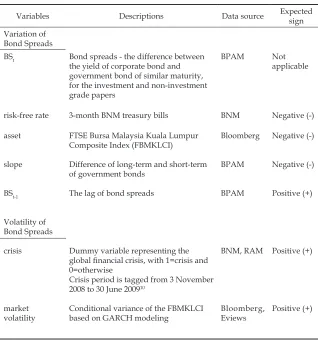
The volatility of the stock market is also included so as to assess the relation and substitutability between the trading of bonds and the equity market. Table 1 below summarises the variables used together with its
description and data source. Appendix I provides additional explanation
and the citation of literature supporting the variables.
4.3 Methodology
Volatility in the return of financial asset instruments is first reported
Table 1: Data Requirement and Source of Data
Variables Descriptions Data source Expected sign Variation of
Bond Spreads
BSt Bond spreads - the difference between
the yield of corporate bond and government bond of similar maturity, for the investment and non-investment grade papers
BPAM Not
applicable
risk-free rate 3-month BNM treasury bills BNM Negative (-) asset
slope
BSt-1
Volatility of Bond Spreads crisis
market volatility
FTSE Bursa Malaysia Kuala Lumpur Composite Index (FBMKLCI)
Difference of long-term and short-term of government bonds
The lag of bond spreads
Dummy variable representing the global financial crisis, with 1=crisis and 0=otherwise
Crisis period is tagged from 3 November 2008 to 30 June 200910
Conditional variance of the FBMKLCI based on GARCH modeling
Bloomberg
BPAM
BPAM
BNM, RAM
Bloomberg, Eviews
Negative (-)
Negative (-)
Positive (+)
Positive (+)
Positive (+)
10 It is observed that the financial crisis that shook the US financial system started in June 2007
regression analysis in the presence of heteroscedasticity provides an
unbiased result. However, the standard errors and confident intervals
estimated will be too narrow thereby, resulting in misleading inferences (Engle, 2001).
In order to treat heteroscedasticity as a variance that can be
modelled, Engle and Bollerslev (1986) introduced the autoregressive conditionally heteroscedastic (ARCH) model which was later extended
by Bollerslev (1986) as the GARCH model. In the GARCH model, the
variance conditional of past situations is expressed as a linear function of the squared past values of the series. The application of the ARCH
and GARCH models on financial time series allows the correction of the deficiencies of least squares. It also allows for the computing of a
prediction for the variance of the error term and this enables researchers
to study the behaviour of the variance (Engle, 2001). In making a
consideration that the data on bond spreads in this study are expected
to exhibit persistent volatility clustering, it is thus justified to employ
the non-linear GARCH model introduced by Bollerslev (1986).
With the GARCH (1,1)11 model being the most popular model in modelling the asset-return volatility, the estimation model in this
study is in line with Rachev, Mittnik, Fabozzi, Focardi, and Jašić (2007)
and hereby also similar to the model used by Manzoni (2002). This is presented below as
∆BSt = α + β1∆risk-free + β2∆asset+ β3 ∆slope + β4∆BSt-1+ɛt (6)
,
+ crisis + market volatility (7)
where the ∆BSt is the change in the relative bond spreads (for the consolidated bond rated AAA, AA, A, BBB, BB, and B with short-term maturity (3 years) and long-short-term maturity (10 years), a total of 10 rating and maturity combination at time t), ∆risk-free is the treasury bill
of Bank Negara Malaysia, ∆asset is the change in the logarithm of the
stock market index, ∆slope is the change in the slope of the yield curve,
∆BSt-1 is the autoregressive term or the lag of spreads which is used to
model how the previous spreads influences future spreads, and crisis
is the dummy variable tagging the 2007/2008 global financial crisis.
The conditional variance term (ht) is modelled by the past shock or news which is measured as the lag of the squared residual from the mean equation that is known as the ARCH term (g1ε2
t-1) and its own
lagged value known as the GARCH term (g2 σt-1) which represents the
last period’s forecast variance. For (7) to be well defined and to ensure
that the conditional variance of the error term (ht) is stationary, g1+g2 must
be close to 1. This model specifies that this period’s variance is formed
by namely: a weighted average of long-term average (the constant), information about volatility which is observed in the previous period arising from some shock or news (ARCH term) and forecast variance acquired from the last period - the GARCH term (Batten & Hogan, 2003).
4.3.1 Modelling the Asymmetry
By construction, the conditional variance in the GARCH model only depends on the modulus of the past variables where, past positive and negative innovations have the same effect on the current volatility.
In other words, good and bad news or shocks have the same effect
(symmetrical) on the volatility of the common GARCH model. This is regarded as one of the drawbacks of the standard GARCH model. Many empirical studies looking at asset returns shows that the conditional asymmetry is a stylised fact where volatility increase due to a price decrease is generally stronger than that resulting from a price increase of the equivalent magnitude (Francq & Zakoian, 2010).
The asymmetric GARCH process for bond spreads, as proposed by Manzoni (2002), provides an alternative approach which is used for checking any level effect that scrutinises whether the observed conditional heteroscedasticity in the data could be better accounted for. Black (1976), in detecting stock market volatility changes, highlights that volatilities tend to be higher after negative shocks than after positive shocks. This phenomenon is referred to as “leverage effect” since it links
the equity value of the firm to the risk of the market. This leverage effect
is explained as and when the price of a stock falls that is when the debt-equity ratio of the company increases which simultaneously increases the risk. This is referred to as the volatility of the stock.
The common GARCH model is deemed to be inappropriate in modelling the asymmetric behaviour of the asset returns hence, the TARCH and EGARCH models are introduced. They are further explained.
• The TARCH model proposed by Zakoian (1994) captures the
followed by higher volatilities, and the conditional variance is expressed as:
where the leverage effect exists if θ> 0.
(8) dt = 1 if εt < 0, and 0 if otherwise
ht = a+ f εt-12 + θε2t-1 dt-1+ φht-1+ut
(9) log(ht) = a+ Σqi=1g1ig(ηt-i) + Σi=1q g2ilog(ht-i)
where εt = √ht ηt and g(ηt) = θηt+g[|ηt| —E|ηt|] are the weighted innovations that model asymmetric effects between the positive and negative asset returns, and θ and g are constants. Both ηt and E[g(ηt)]are zero mean IID sequences with continuous distribution.
Hence, E[g(ηt)] = 0. Based on Rachev et al. (2007), the function of
g(ηt) can be rewritten as:
(10) (θ+ g) ηt– gE(|ηt|) if ηt ≥ 0
(θ+ g) ηt– gE(|ηt|) if ηt < 0 g(ηt) =
{
so that θ + g and θ - g reflect the asymmetry in response to positive
and negative innovations. Apparently, the model is nonlinear if g ≠ 0. If θ < 0, a positive return shock or surprise will increase the volatility lesser than a negative one of the same magnitude. This phenomenon is referred to as leverage effect as explained earlier.
5. Empirical Results and Discussion
5.1 Descriptive Statistics
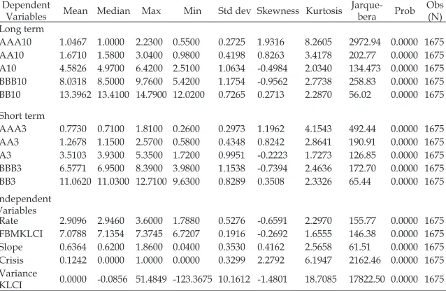
The descriptive statistics constructed for all the dependent (bond spreads of different maturity and ratings) and independent variables are presented in Table 2 below.
The mean for long term and short term bond spread increases as the rating decreases. This indicates that risk premium increases between the investment grade and non-investment grade bond. The risk-return trade off also becomes apparent where it is observed that the larger the standard deviation, the higher the credit spreads is. Generally, the spreads presents positive skewness except for A10, BBB10 and BBB3. Positive skewness implies that the left tail of the loss distribution (for a
• The EGARCH model proposed by Nelson (1991) specifies the
Dependent
Variables Mean Median Max Min Std dev Skewness Kurtosis Jarque-bera Prob Obs (N) Long term
AAA10 1.0467 1.0000 2.2300 0.5500 0.2725 1.9316 8.2605 2972.94 0.0000 1675 AA10 1.6710 1.5800 3.0400 0.9800 0.4198 0.8263 3.4178 202.77 0.0000 1675 A10 4.5826 4.9700 6.4200 2.5100 1.0634 -0.4984 2.0340 134.473 0.0000 1675 BBB10 8.0318 8.5000 9.7600 5.4200 1.1754 -0.9562 2.7738 258.83 0.0000 1675 BB10 13.3962 13.4100 14.7900 12.0200 0.7265 0.2713 2.2870 56.02 0.0000 1675 Short term
AAA3 0.7730 0.7100 1.8100 0.2600 0.2973 1.1962 4.1543 492.44 0.0000 1675 AA3 1.2678 1.1500 2.5700 0.5800 0.4348 0.8242 2.8641 190.91 0.0000 1675 A3 3.5103 3.9300 5.3500 1.7200 0.9951 -0.2223 1.7273 126.85 0.0000 1675 BBB3 6.5771 6.9500 8.3900 3.9800 1.1538 -0.7394 2.4636 172.70 0.0000 1675 BB3 11.0620 11.0300 12.7100 9.6300 0.8289 0.3508 2.3326 65.44 0.0000 1675
Independent
Variables
Rate 2.9096 2.9460 3.6000 1.7880 0.5276 -0.6591 2.2970 155.77 0.0000 1675
FBMKLCI 7.0788 7.1354 7.3745 6.7207 0.1916 -0.2692 1.6555 146.38 0.0000 1675
Slope 0.6364 0.6200 1.8600 0.0400 0.3530 0.4162 2.5658 61.51 0.0000 1675 Crisis 0.1242 0.0000 1.0000 0.0000 0.3299 2.2792 6.1947 2162.46 0.0000 1675 Variance
KLCI 0.0000 -0.0856 51.4849 -123.3675 10.1612 -1.4801 18.7085 17822.50 0.0000 1675 Table 2: Descriptive Statistics for Dependent and Independent Variables
Note: The lag for each bond spreads is not shown as its characteristics are not as meaningful as the spreads itself. However, it is included as one of the independent variables in the mean variation of the GARCH analysis to investigate the influence of previous trend of the spread in the following day.
long position) possesses more probability than a normal one (Gujarati, 2003). Bond spreads is also leptokurtic, given the large kurtosis values, in most cases (except for A10, A3 and BBB3), which is characterised by a fairly large likelihood of small spreads, together with a small chance of large bond spreads. According to Manzoni (2002), this characteristic
is in line with the specific feature of credit risk that is subjected to small frequent variations and rare large variations. In summary, the data
distributions of the bond spreads present signs of the characteristic of fat-tailed behaviour where the Jarque-Bera statistic for the null hypothesis of normality is far beyond the critical value of 1 per cent level, suggesting that these series are far from being normal distributions.12 The plots for
12 Due to the non-stationarity of the time-series data, the Augmented Dickey-Fuller (ADF)
investment and non-investment grades bonds are presented in Figures 3(a) and 3(b) respectively.
Figure 3(a) (i) and (ii): Bond Spreads of Investment Grades (AAA, AA, A, BBB) Grouped by Maturity (at levels)
(ii) 3-year bond spreads
Figure 3(b) (i) and (ii): Bond Spreads of Non-Investment Grade (BB) Grouped by Maturity (at levels)
Volatility of the spreads, as presented by the standard deviation, also increases as the rating decreases even though the volatility of BBB bonds for both long term and short term is slightly higher than those
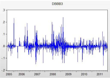
rated BB. In addition to that, the phenomenon of volatility clustering
is also observable when the changes in spreads are plotted for (a) investment grade bonds and (b) non-investment grade bonds, as shown in Figure 4.
Figure 4(a) (i) and (ii): Time Series Plot of Changes in Investment Grade Bond Spreads
(i) 10-year bond spreads
(ii) 3-year bond spreads
5.2 Estimation Results
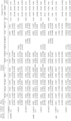
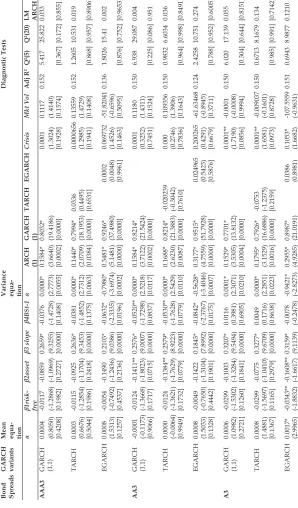
Table 3 presents the estimation results of the investment and non-investment grade bonds which are grouped by maturity of long term
(Table 3(a)) and short term (Table 3(b)). In the Table, the three different
types of models, GARCH (1.1), TARCH and EGARCH, are presented for each rating, from AAA to BB. For each of the model shown in the
Table, the first panel presents the mean equation where the main four
(4) variables of risk: free rate, asset return, slope and the lag of spreads, are regressed against the variation of bond spreads. The second panel presents the variance equation where apart from the past shocks and
forecast variance, the dummy representing global financial crisis and
stock market volatility are included to analyse the volatility of bond spreads.
In order to ensure that all the models are fit for hypothesis testing,
diagnostic tests are undertaken and this is presented in the third panel of the Table. The presence of serial correlation of the estimated residuals as seen from the estimation is tested by using the Ljung-Box Q-statistics for lag 2 which is applied to the squared standardised residuals. The Q-statistics indicates that the null hypothesis of no serial correlation
cannot be rejected hence, the mean equation is not mis-specified. In order
to test whether any remaining heteroscedasticity exists in the estimation
model, the ARCH LM specifications, with all lags (up to lag 2), is carried
out. The observed R-squared (Obs*R-squared) statistics indicate that the ARCH effect is eliminated with the high value of the chi-square probability. Hence, all models do not suffer any serial correlation and
further heteroscedasticity effect. This makes it a fit and robust model
for hypothesis testing which hereby meets the research objectives. The following discussion is based on the mean and variance equations of the estimation results taken from the total of 10 ratings and maturity combination.
5.2.1 What Drives Bond Spreads?
The first panel on the left hand side of Table 3(a) and (b) presents the mean equation of the model which examines the factors influencing the variation of bond spreads for each of the rating. Similar to the finding
on sukuk spreads by Rahman et al. (2013), the most influencing factor
be significantly negative for bond spreads of longer maturity that has the rating of A and below. However, this variable is not significant to
the high rating of long term bond (AAA and AA) and to the short term bond spreads, except for BB3.
On looking at the term structure of credit spreads and its association with changes in interest rates, it appears that the theory proposed by Sundaram and Das (2010) is applicable in explaining this phenomenon. According to the theory, for short maturities, default is an unlikely event,
hence spreads is low. However as maturity lengthens, there is sufficient
time for the bond to default, given the vulnerable state of the economy of which the interest rate is subjected to change, and that the default
probability of the firm is higher, as reflected by a higher spreads. This significant and negative relation of this variable is consistent with the
two-factor theoretical framework proposed by Longstaff and Schwartz (1995) as well as other studies (particularly Manzoni, 2002; Batten &
Hogan, 2003; Batten et al., 2006). As for the insignificance of the risk
free rate with the high rating of long term bond, intuitively speaking, it is regarded that bonds of high rating tend to be somehow resilient to the drastic movement of the interest rates.
The significance of the slope variable strongly supports the basic understanding that bond spreads is very much influenced by the
anticipated movements of the future rate and it is in line with the
findings of previous studies (Avramov et al., 2007 Batten et al., 2006; Boss
& Scheicher, 2002; Hattori et al., 2001; Lepone & Wong, 2009; Manzoni, 2002; Miloudi & Moraux, 2009; Rahman et al., 2013; Naifar & Mseddi,
2013; Yap & Gannon, 2007).
Other variables representing the equity market return and the asset
factor, show no significance in all ratings, except for AAA3 which stands at a higher level of significance. With the view that the significance is
only for one rating, it is thus deduced that this factor does not actually
contribute to variation in bond spreads. This finding is inconsistent with the initial finding made by Longstaff and Schwartz (1995) and
with the main literature discussed (see Appendix 1). Nevertheless,
similar findings are seen in Rahman et al. (2013) who suggest that the
Malaysian bond market that is established since the early 1990s is much more stable. They also assert that the Malaysian market possesses its
own market niche where trading of bonds may not be influenced by the
changes observed of the return in the stock market. Finally, in looking at the previous trading patterns measured by the lags of the bond spreads,
Bond Spreads GARCH variants Mean equation Variance equation
Diagnostic Tests α β1risk- free β2asset β3 slope 4BSt-1 α
ARCH (1) GARCH (1)
TARCH
EGARCH
Crisis
Mkt Vol
Adj R2
Q
2(5)
Q
2(20)
LM ARCH
AAA10
GARCH (1,1)
-0.0003* -0.0160 -0.0160 -0.2037* -0.0292 0.0000 0.2382* 0.7778* 0.0000 0.2046 0.191 5.1936 20.031 0.116 (-0.6317) (-1.6431) (-0.1866) (-10.6305) (-0 .7 76 5) (-1.3110) (-4.7484) (-23.0467) (1.0008) (1.5335) [0.5276] [0.1004] [0.852] [0.000] [0.4375] [0.1899] [0.000] [0.000] [0.3169] [0.1252] [0.393] [0.456] [0.7339] TARCH -0.0002 -0.0161** -0.0059 -0.2182* -0.0238 0.0000 0.2724* 0.7713* -0.0611 0.0001 0.2299 0.201 5.705 19.383 0.063 (-0.4835) (-1.6494) (-0.0678) (-10.9522) (-0 .6 28 6) (1.3473) (3.9173) (22.7223) (-0.7816) (1.0519) (1.5704) [0.6288] [0.0991] [0.9459] [0.000] [0.5296] [0.1779] [0.0001] [0.000] [0.4345] [0.2929] [0.1163] [0.336] [0.497] [0.8015] EGARCH -0.0003 -0.0025 -0.1179 -0.0803* -0.0062 -0.6112* 0.3723* 0.9499* 0.0298 0.0522 -26.8863 0.084 8.0561 14.237 0.231 (-0.8427) (-0.4840) (-0.9423) (-5.5572) (-0 .1 56 3) (-3.5713) (5.1858) (50.6254) (0.7008) (1.3185) (-0.3256) [0.3994] [0.6284] [0.3460] [0.000] [0.8758] [0.0004] [0.000] [0.000] [0.4834] [0.1873] [0.7447] [0.153] [0.818] [0.6307] AA10
GARCH (1,1)
0.0001 -0.0020 0.0013 -0.0359* -0.0113 0.0000* 0.2142* 0.8494* 0.0000 -0.1282* 0.038 9.5865 19.824 0.000 (0.4814) (-0.8543) (0.0411) (-3.6715) (-0 .2 69 7) (9244.3100) (4.0082) (30.1977) (0.5377) (-35.2267) [0.6302] [0.3929] [0.9672] [0.0002] [0.7874] [0.000] [0.0001] [0.000] [0.5913] [0.000] [0.088] [0.469] [0.9853] TARCH 0.0001 0.0002 0.0128 -0.0340* -0.0120 0.0000* 0.2311* 0.8499* -0.0375 0.0000 -0.1302* 0.034 14.999 19.847 0.001 (0.5551) (0.0709) (0.3852) (-3.5105) (-0 .2 85 6) (7515.3100) (3.6703) (31.0948) (-0.6167) (0.5505) (-26.3306) [0.5788] [0.9435] [0.7001] [0.0004] [0.7752] [0.000] [0.0002] [0.000] [0.5374] [0.5819] [0.000] [0.01] [0.468] [0.9700] EGARCH -0.0004 -0.0038 -0.1606 -0.0588* 0.0000 -0.5357* 0.3743* 0.9587* 0.0314 0.0399 -95.4723 0.058 4.0251 8.5266 0.001 (-1.2622) (-0.7151) (-1.1239) (-4.8458) (-0 .0 01 1) (-3.2690) (5.6227) (55.7137) (0.7505) (1.0347) (-1.0134) [0.2069] [0.4745] [0.2610] [0.000] [0.9992] [0.0011] [0.000] [0.000] [0.4529] [0.3008] [0.3109] 0.546 0.988 0.9752 A10
GARCH (1,1)
EGARCH 0.0022** -0.0638* -0.0191 -0.3698* -0.0118 -1.0349* 0.4197* 0.8967* 0.0179 0.130169 -141.0073 0.280 0.8255 4.3314 0.005 (1.9393) (-2.6597) (-0.2077) (-9.4432) (-0 .3 30 6) (-2.5268) (4.4770) (18.3191) (0.4041) (1.627) (-0.9762) [0.0525] [0.0078] [0.8354] [0.0000] [0.7409] [0.0115] [0.0000] [0.0000] [0.6862] [0.1037] [0.3290] [0.975] [1.000] [0.9449] BBB10
GARCH (1,1)
0.0012 -0.1914* -0.2137 -0.4681* 0.0012 0.0001** 0.5005* 0.6499* 0.0002 -0.1040 0.286 7.8956 19.911 0.002 (0.8556) (-3.9373) (-1.2731) (-10.1244) (0.0370) (1.9511) (2.1332) (6.1483) (1.0466) (-0.8562) [0.3922] [0.0001] [0.2030] [0.0000] [0.9705] [0.0510] [0.0329] [0.0000] [0.2953] [0.3919] [0.162] [0.463] [0.9669] TARCH 0.0010 -0.1956* -0.2216 -0.4685* -0.0002 0.0001* 0.4717* 0.6500* 0.0715 0.00026 -0.101889 0.285 1.1688 3.4317 0.001 (1.1121) (-3.9775) (-1.3416) (-10.4017) (-0 .0 05 8) (2.2137) (2.7470) (6.6903) (0.2342) (0.9478) (-0.8632) [0.2661] [0.0001] [0.1797] [0.0000] [0.9954] [0.0268] [0.0060] [0.0000] [0.8148] 0.3433] [0.3880] [0.948] [1.000] [0.979] EGARCH 0.0024 -0.0896* -0.1796 -0.5068* 0.0353 -1.0416* 0.4669* 0.8918* -0.0414 0.570441 -257.2807 0.301 0.5632 2.0125 0.016 (1.6285) (-2.7777) (-1.5869) (-9.2182) (1.0817) (-2.2544) (3.2216) (16.1186) (-0.6453) (1.0803) (-1.1254) [0.1034] [0.0055] [0.1125] [0.0000] [0.2794] [0.0242] [0.0013] [0.0000] [0.5187] [0.2800] [0.2604] [0.990] [1.000] [0.9006] BB10
GARCH (1,1)
Ta bl e 3 (b ) Bond Spreads GARCH variants Mean equa
-tion
Variance equa
-tion Diagnostic Tests α β1risk- free β2asset β3 slope β4BSt-1 α
ARCH (1) GARCH (1)
TARCH EGARCH Crisis Mkt Vol Adj R 2Q 2(5) Q 2(20)
LM ARCH
AAA3
GARCH (1,1)
0.0004 -0.0117 -0.0859 0.2659* -0.0376 0.0000* 0.1584* 0.8032* 0.0001 0.1117 0.152 5.417 25.822 0.033 (0.8050) (-1.2868) (-1.0969) (9.3255) (-1.4728) (2.7773) (3.6640) (19.4186) (1.3024) (1.4140) [0.4208] [0.1982] [0.2727] [0.0000] [0.1408] [0.0055] [0.0002] [0.0000] [0.1928] [0.1574] [0.367] [0.172] [0.855] TARCH 0.0003 -0.0115 -0.0925 0.2636* -0.0381 0.0000* 0.1440* 0.7994* 0.0336 0.0000656 0.13559 0.152 1.2605 10.531 0.019 (0.6676) (-1.2854) (-1.1704) (9.3453) (-1.4852) (2.7312) (2.0709) (18.1953) (0.4495) (1.2985) (1.4729) [0.5044] [0.1986] [0.2418] [0.0000] [0.1375] [0.0063] [0.0384] [0.0000] [0.6531] [0.1941] [0.1408] [0.868] [0.957] [0.8906] EGARCH 0.0008 -0.0054 -0.1490 0.2103* -0.0632* -0.7980* 0.3481* 0.9246* 0.0002 0.069732 -51.82041 0.136 1.8026 15.41 0.002 (1.5313) (-0.7492) (-1.2436) (9.0386) (-2.3335) (-3.6974) (5.1481) (37.4980) (0.0048) (1.4526) (-0.6596) [0.1257] [0.4537] [0.2136] [0.0000] [0.0196] [0.0002] [0.0000] [0.0000] [0.9961] [0.1463] [0.5095] [0.876] [0.752] [0.9653] AA3
GARCH (1,1)
-0.0001 -0.0124 -0.1411** 0.2576* -0.0520** 0.0000* 0.1584* 0.8214* 0.0001 0.1180 0.150 6.938 29.087 0.004 (-0.1173) (-1.3668) (-1.8023) (9.0007) (-1.7298) (2.5218) (3.7122) (21.5424) (0.3252) (1.4311) [0.9066] [0.1717] [0.0715] [0.0000] [0.0837] [0.0117] [0.0002] [0.0000] [0.7451] [0.1524] [0.225] [0.086] 0.951 TARCH 0.0000 -0.0124 -0.1384** 0.2579* -0.0530** 0.0000* 0.1688* 0.8214* -0.020239 0.000 0.109356 0.150 0.9832 6.6034 0.036 (-0.0064) (-1.3621) (-1.7629) (8.9223) (-1.7628) (2.5429) (2.6230) (21.3883) (-0.3042) (0.2746) (1.3906) [0.9949] [0.1732] [0.0779] [0.0000] [0.0779] [0.0110] [0.0087] [0.0000] [0.7610] [0.7836] [0.1643] [0.964] [0.998] [0.8491] EGARCH 0.0008 -0.0049 -0.1422 0.1845* -0.0842* -0.5628* 0.3177* 0.9515* 0.024965 0.200265 -61.63468 0.124 2.4258 10.751 0.274 (1.5033) (-0.7650) (-1.3104) (7.8992) (-2.3767) (-3.4046) (4.7559) (51.7928) (0.5423) (0.4291) (-0.8945) [0.1328] [0.4442] [0.1901] [0.0000] [0.0175] [0.0007] [0.0000] [0.0000] [0.5876] [0.6679] [0.3711] [0.788] [0.952] [0.6005] A3
GARCH (1,1)
[0.0027] [0.0597] [0.0966] [0.0000] [0.8043] [0.0047] [0.0000] [0.0000] [0.3691] [0.0953] [0.3355] [0.983] [0.983] [0.728] BBB3
GARCH (1,1)
0.0006 -0.0181 -0.0698 0.3696* 0.0590** 0.000** 0.1979* 0.7328* 0.0002** -0.0809 0.147 11.847 17.097 0.026 (1.1479) (-0.6016) (-0.8480) (10.1979) (1.8634) (1.9174) (3.9381) (13.0429) (1.7080) (-1.1373) [0.2510] [0.5475] [0.3964] [0.0000] [0.0624] [0.0552] [0.0001] [0.0000] [0.0876] [0.2554] [0.037] [0.647] [0.8727] TARCH 0.0007 -0.0187 -0.0647 0.3707* 0.0572* 0.0001** 0.2075* 0.7348* -0.0242 0.0002** -0.078733 0.147 0.4778 3.2934 0.0225 (1.3276) (-0.6249) (-0.7873) (10.1978) (1.8078) (1.8710) (3.0642) (12.9443) (-0.2656) (1.6940) (-1.1153) [0.1843] [0.5321] [0.4311] [0.0000] [0.0706] [0.0613] [0.0022] [0.0000] [0.7906] [0.0903] [0.2647] 0.993 [1.000] [0.8808] EGARCH 0.0016** -0.0228 -0.0823 0.3349* 0.0251 -1.2541* 0.3276* 0.8574* 0.0127 0.161667 -244.7104 0.148 0.1474 2.6284 0.002 (1.9455) (-0.8541) (-0.8195) (7.9281) (0.5700) (-2.1934) (5.2809) (10.9681) (0.2259) (1.5687) (-1.1979) [0.0517] [0.3931] [0.4125] [0.0000] [0.5687] [0.0283] [0.0000] [0.0000] [0.8213] [0.1167] [0.2309] [1.000] [1.000] [0.9685] BB3
GARCH (1,1)
in bond spreads. This finding is also similar to the results obtained by
Rahman et al. (2013) who examined sukuk spreads.
5.2.2 Main Component of Bond Spreads Volatility
The variance equation of each bond spreads which examines the volatility is presented in the second and middle panels of Tables 3(a)
and (b). The volatility is mainly influenced by the ARCH and GARCH
terms and this in turn, represents the news or shock and forecast variance
respectively. This finding is similar to studies which applied the GARCH
model as discussed in Section 3 above. The dummy crisis variable used
here appears to be significant standing at 10 per cent level of significance
only for the short term and lower investment grade of bond spreads (A3,
BBB3). However, the extremely small value of the coefficient indicates that the bond is not susceptible to the 2007/8 financial crisis.
In looking at the stock market volatility, the empirical results produced here fail to establish any significant relation with bond
spread volatility. Even though the z-statistics of the regression model
shows that the variable is significantly different from zero for AA10, the extremely small values of the coefficient do not provide a meaningful interpretation for its significance.
Extending the analysis to evaluate on the asymmetric response to past shocks, the TARCH and EGARCH models were regressed against the additional variables hereby representing the crisis dummy and stock
market volatility. The coefficients obtained when using the TARCH and EGARCH models appear to be not statistically significant for all
ratings and maturity. Hence, no evidence of asymmetric response in the volatility of bond spreads is documented.
6. Conclusion
The general objective of the research is to analyse the trend, behaviour
and influencing factors of the variation of credit spreads in the Malaysian
bond market. Credit spreads provides information which can enable
the assessing of credit risk. It is widely used in the pricing of bonds
and in the analysing of variations thus, it is essential to be used in the management of risk and for sound decision making.
Adopting the two-factor framework of Longstaff and Schwartz (1995), this study expands on the work of Rahman et al. (2013) by
aiming to unveil the factors which influence the variation of bond
bond market. By applying the GARCH (1,1) model, this study finds that the anticipation of the interest rate (slope) is the most significant
variable for explaining the variation of the bond spreads, apart from the
movement of the interest rate for several ratings and maturity. In order to examine the impact of the recent 2007/2008 global financial crisis,
the dummy variable which represents the crisis is included in analysing the volatility of the bond spreads. Further, in exploring whether the increasing pattern of the volatility of future stock returns could raise the bond risk premium, the stock market volatility is also considered. By applying the extended model of GARCH in analysing the asymmetrical properties of bond spread volatility, the TARCH and EGARCH models
have been employed. Nonetheless, the insignificance of the respective TARCH and EGARCH coefficients indicate that there is no evidence of
asymmetric response in the volatility of bond spreads.
This study is among the first few to analyse the movement of bond
spreads in the Malaysian bond market given that spreads analysis is often used as a measure of credit risk and as a signal of probability
of default. Apart from enriching the financial economics literature in Malaysia, the findings of this study are expected to benefit issuers,
traders and portfolio managers. For the issuers, the knowledge of how the trend of spreads works can enable them to compute a competitive pricing for bonds. As the variation in spreads is able to signal the risk tolerance for investing into corporate bonds vis-a-vis government bonds, a close observation on the recent variation of bond spreads is vital. This can ensure that new bond issuance will be priced in such a way that the
cost is manageable for issuers and favourable to investors. In addition,
since the component of the yield pricing consists of the risk free rate plus
some spreads, the findings can also provide some practical insights on
the factors which could influence the spreads. Fabozzi (2007) asserts that
a yield/spread pick up trade represents the most common secondary trading technique which requires traders to compare the spreads against relatively similar rating and maturity of bonds. By comparing the spreads of different bonds with similar credit rating, duration and outlook, it can be noticed that bonds with a higher spreads would be a better buy, given that the same level of risk is compensated higher by
one bond than the other. Hence, knowing what factors would influence
the variation in bond spreads is important.
On the other hand, depending on their trading and investment objectives, traders and fund managers may find the information
it allows them to gauge the expected changes in the spreads level within the market and also to notice which bond rating (at certain maturity) is currently being sought after. This is important, given that the trading of bond is normally undertaken over the counter where spreads is used as a common platform for comparing bonds of similar rating and maturity.
Another important implication of this study is the similar findings of the factors influencing the sukuk and bond spreads. This leads to the need to highlight the notion of, “In terms of trading based on spreads, sukuk and bonds are treated similarly by the market players”. This similarity is subject to the risk premium assessment which is based on spreads and which may be due to the fact that sukuk is not only demanded by
the Islamic financial institutions, but also by the non-Islamic financial
institutions. As such, for fund managers managing non-Shariah compliant bond portfolios, comparing the spreads between these two instruments allows them to have a common platform to contrast and compare the compensation of risks with the purchase of sukuk and bonds.
Finally, given that these findings are solely focused on the Malaysian bond market, a further and extended research in modelling the conditional variance of other neighbouring countries such as the
Singaporean and Indonesian bond markets is believed to be of interests
to many researchers as well as industry practitioners.
References
Ahmad, N., Muhammad, J., & Masron, T.A. (2009). Factors influencing yield spreads of the Malaysian bonds. Asian Academy of Management Journal, 14(2), 95-114.
Asian Development Bank (ADB). (2015). Asia Bond Monitor - March 2015. Available at http://asianbondsonline.adb.org (accessed on April 2015) Avramov, D., Jostova, G., & Philipov, A. (2007). Understanding changes in
corporate credit spreads. Financial Analysts Journal, 63(2), 90-105.
Bank of International Settlements (BIS) Quarterly Review, June 2012. Available at <http://www.bis.org/statistics/secstats.htm>
Batten, J.A., Fetherston, T.A., & Hoontrakul, P. (2006). Factors affecting yield of emerging market issuers: Evidence from the Asia-Pacific region. Journal of International Financial Markets, Institutions and Money, 16,57-70.
Batten, J.A., & Hogan, W.P. (2003). Time variation in the credit spreads on Australian Eurobonds. Pacific-Basin Finance Journal, 11,81-99.
Bollerslev, T. (1986). Generalized autoregressive conditional heteroscedasticity. Journal of Econometrics, 31, 307-327.
Black, F., & Cox, J. (1976). Valuing corporate securities: Some effects of bond indenture provisions. Journal of Finance, 31,351-367.
Black, F. (1976). Studies of stock price volatility changes. Proceedings of the 1976 Meetings of the American Statistical Association, Business and Economical Statistics Section. pp. 177-181.
Boss, M., & Scheicher, M. (2002). The determinants of credit spread changes in the Euro Area. Working Paper, No. 12, Bank of International Settlements (BIS), 181-199.
Bond Pricing Agency Malaysia (BPAM). (2009). Pricing Methodology: Sukuk Valuation – Theory and Practice. Materials presented at the Quantitative Islamic Finance and Takaful Seminar, Universiti Kebangsaan Malaysia, Bangi, Malaysia in July 2009.
Connolly, R., Stivers, C., & Sun, L. (2005).Stock market uncertainty and the stock-bond return relation. Journal of Financial and Quantitative Analysis, 40(1),161-194.
Davies., A. (2007). Credit spread determinants: An 85 years perspective. Journal of Financial Markets, 11, 180-197.
Demchuk, A., & Gibson, R.. (2006). Stock market performance and the term structure of credit spreads. Journal of Financial and Quantitative Analysis, 41, 863-887.
Duffee, D., & Singleton, K. (1999). Modelling term structures of defaultable bonds. Review of Financial Studies, 12, 687-720.
Engle, R., & Bollerslev, T. (1986). Modeling the persistence of conditional variances. Econometric Review, 5(1), 1-50.
Engle, R. (2001). GARCH 101: The use of ARCH/GARCH models in applied Econometrics. Journal of Economic Perspectives, 15(4) 157-168.
Elton, E.J., Gruber, M.J., Agrawal, D., & Mann, C. (2001). Explaining the rate spread on corporate bonds. Journal of Finance, LVI(1), 247-277.
Fabozzi, F. (2000). Bond Markets, Analysis and Strategies. New Jersey: Prentice Hall.
Fabozzi, F. (2007). Fixed Income Analysis. New Jersey: John Wiley & Sons, Inc.
Francq, C., & Zakoian, J-M. (2010). GARCH Models: Structure, Statistical Inference
and Financial Applications. UK: John Wiley and Sons Ltd.
Fleming, J., Kirby, C., & Ostdiek, B. (2001). The economic value of volatility timing. The Journal of Finance, 56(1), 329-352.
Giesecke, K., Longstaff, F.A., Schaefer, S., & Strebulaev, I. (2011). Corporate bond default risk: A 150-year perspective. Journal of Financial Economics, 102. 233-250.
Hattori, M., Koyama, K., & Yonetani, T. (2001). Analysis of credit spread in
Japan’s corporate bond market. The Changing Shape of Fixed Income Markets:
A Collection of Studies by Central Bank Economists, BIS Papers, (5), 113-46.
Hibbert, A.M., Pavlova, I., Barber, J.B., & Dandapani, K. (2011) Credit spread changes and equity volatility: Evidence from daily data. The Financial Review, 46, 357-383.
Jarrow, R.A., Lando, D., & Turnbull, S. (1997). A Markov model for the term structure of credit risk spreads. Review of Financial Studies, 10, 481-523. Jones, C.P. (2007). Investment. John Wiley & Sons (Asia) Pte Ltd.
Krainer, J. (2004). What determines the credit spread? Federal Reserve Bank of San Francisco (FRBSF) Economic Letter, No.36.
Landschoot, A.V. (2008). Determinants of yield spreads dynamics: Euro versus US dollar corporate bonds. Journal of Banking & Finance, 32. 2597-2605. Longstaff, F., & Schwartz, E. (1995). A simple approach to valuing risky fixed
and floating rate debt. Journal of Finance, 50(3),789-819.
Lepone, A., & Wong, A. (2009). Determinants of credit spread changes: Evidence from the Australian bond market. The Australasian Accounting Business & Finance Journal, 3(2), 26-35.
Li, Y. (2003). Treasury Yields, Equity Returns, and Credit Spread Dynamics. Unpublished PhD dissertation, University of Toronto, Canada.
Mandlebrot, B.B. (1963). The variation of certain speculative prices. Journal of Business 36, 394-419.
Manzoni, K. (2002). Modelling credit spreads: An application to the Sterling Eurobond market. International Review of Financial Analysis, 11, 183-218. Merton, R.C. (1974). On the pricing of corporate debt: The risk structure of
interest rates. Journal of Finance, 29, 449-470.
Morris, C., Neal, R., & Rolph, D. (1998). Credit spreads and interest rates: A
cointegration approach (No. 98-08). Federal Reserve Bank of Kansas City.
Miloudi, A., & Moraux, F. (2009). Relations between the corporate credit spreads, treasury yields and the equity market. International Journal of Business, 14(2), 105-122.
Naifar, N., & Mseddi, S. (2013). Sukuk spreads determinants and pricing model methodology. Afro-Asian Journal of Finance and Accounting, 3(3), 241-257. Nakashima, K., & Saito, M. (2009). Credit spreads on corporate bonds and
macroeconomy in Japan. Journal of the Japanese and International Economies, 23, 309-331.
Nelson, D. (1991). Conditional heteroskedasticity in asset returns: A new approach. Econometrica, 59, 347-370.
Pedrosa, M., & Roll, R. (1998). Systematic risk in corporate bond credit spreads. Journal of Fixed Income, 8(3),7-26.
Rachev, S.T., Mittnik, S., Fabozzi, F.J., Focardi, S.M., & Jašić, T. (2007). Financial
Econometrics: From Basics to Advanced Modelling Techniques. USA: John
Rahman, S. (2003). Analysis of Credit Spread in Malaysian Corporate Bond Market. Unpublished master dissertation, University Putra Malaysia, Kuala Lumpur.
Rahman, M.P., & Omar, M.A. (2012). Factors Influencing the Excess Returns of Sukuk: An Empirical Analysis on USD Denominated Sukuk Issued by Corporations in the Gulf Cooperation Council (GCC). Paper presented in the 3rd Gulf Research Meeting, University of Cambridge, Cambridge, United
Kingdom on 7 July 2012.
Rahman, M.P., Omar, M.A., & Kassim, S.H. (2013). An application of GARCH modelling on the Malaysian sukuk spreads. Journal of Islamic Finance, 2(2), 26-37.
Rahman, M.P., Omar, M.A., Kassim, S.H., & Sutan, E.H. (2013). Understanding investors behaviour from the variation of sukuk spreads. Islamic Finance News, 11, 19-20.
RAM Rating Services Bhd. (2010). Corporate Default and Rating Performance Study (1999-2009). Kuala Lumpur: Author.
Securities Commission (2014). Malaysian ICM Bulletin. January-June 2014. 9(1). Sundaram, R., & Das, S. (2010). Derivatives. United Kingdom: McGraw-Hill
Higher Education.
Tsuji, C. (2005). The credit-spread puzzle. Journal of International Money and Finance, 24(7), 1073-1089.
Yap, C.J., & Gannon, G. (2007). Factors Affecting the Credit Spreads Behavior of USD Denominated Malaysian Bonds. Paper presented in 20th Australasian Finance and Banking Conference 2007 Paper. Available at http://ssrn. com/abstract=1009535 or http://dx.doi.org/10.2139/ssrn.1009535 (accessed on 20 October 2011)
No Influencing Factors Relation and impact Related literature
1 Interest rate
factor Generally, from the perspective of demand and supply, an increase in interest rates may cause the supply of corporate bonds to reduce, causing the yields to fall and hence reduces the spreads. Alternatively from another economic point of view, an increase in interest rates will likely increase the yields of treasury bonds and as this increase will not be proportionately equivalent to the increase in the yields of corporate bonds, spreads will decrease. Hence, a negative relation between the spreads and interest rate factor.
Ahmad et al. (2009), Avramov et al. (2007), Batten and Hogan (2003), Batten et al. (2006), Boss and Scheicher (2002), Davies (2007), Demchuk and Gibson (2006), Li (2003), Landschoot (2008), Lepone and Wong (2009), Longstaff and Schwartz (1995), Giesecke et al (2011), Manzoni (2002), Miloudi and Moroux (2009), Morris et al. (1998), Rahman (2003),
Yap and Gannon (2007),
Tsuji (2005)
2 Asset factor As the asset factor represents
the value of the firm, an increase in the firm’s value
increases the ability of the
firm to service its debt, hence
lowering the probability of the
firm defaulting in its obligation
towards bond holders. Hence, the asset factor is found to have a negative relation with spreads.
Ahmad et al. (2009), Avramov et al. (2007), Batten and Hogan (2003), Batten et al. (2006), Boss and Scheicher (2002), Davies (2007), Demchuk and Gibson (2006), Li (2003), Landschoot (2008), Lepone and Wong (2009), Longstaff and Schwartz (1995), Giesecke et al. (2011), Manzoni (2002), Miloudi and Moroux (2009), Morris et al. (1998), Tsuji (2005),
Rahman (2003), Yap and
Gannon (2007)
Appendix I: Identification of Influencing Factors for the Movement of
No Influencing Factors Relation and impact Related literature 3 Slope The difference between the
long-term and short-term government rate is called slope and provides signal on the expectations of future short term rate and indicates the overall economic health. An increasing slope signals the anticipated increase in the short term rate, which may cause the increase in the yield of the government papers, hence reducing the spreads.
Avramov et al. (2007), Batten et al. (2006) Boss and Scheicher (2002) Hattori et al. (2001), Lepone and Wong (2009), Manzoni (2002), Miloudi and Moraux (2009), Naifar and Mseddi
(2013), Yap and Gannon
(2007)
4 Lag of bond
spreads The previous spreads provides a basis for determining the spreads of a corporate bond, which possesses similar rating and maturity. Being a standard procedure in gauging the current market appetite, previous studies have documented a positive relation of this factor with the spreads.
Batten and Hogan (2003), Hattori et al. (2001), Manzoni (2002), Rahman
(2003), Yap and Gannon