SOFTWARE TOOLSET TO ENABLE IMAGE CLASSIFICATION OF
EARTHQUAKE DAMAGE TO ABOVE-GROUND INFRASTRUCTURE
Anahid BEHROUZI1*, Maria PANTOJA2* (*equal contributors)
ABSTRACT
A critical task after a significant earthquake is determining the extent of damage to infrastructure networks. The decision-making process to dispatch emergency, repair, and in-field reconnaissance teams depends on whether road/railways and bridges are passible. Another concern is the rapid identification and resolution of physical disruptions to large-volume gas and water pipeline systems.
After large seismic events, citizens, amateur photographers, and journalists now post thousands of photographs to formal/social media platforms. In the past, these images would have had to be reviewed by trained volunteers or expert engineers to evaluate whether: road/rail ways were significantly impacted by ground fracture, heaving, slope failure, or rock slides; bridges experienced severe damage or partial-to-complete collapse; and pipeline systems were interrupted by differential ground movement or liquefaction. The manual review of large image-sets for assessing damage has shown to be inefficient and, in cases, error-prone.
This paper presents an automatic and rapid approach, based on computer vision techniques, to assessing damage to above-ground infrastructure networks via images uploaded in the immediate aftermath of the earthquake. The authors developed an algorithm based on deep learning (DL) that automatically tags images. Progress to date shows the algorithm correctly assigns individual tags to 92% of roadway images exhibiting cracking (of varying directionality and severities) and 80% of railways affected by horizontal offset (lateral translation). These results show promise and future research efforts entail tagging both of the aforementioned damage types in a single image.
Keywords: Image classification software; virtual reconnaissance; infrastructure network damage; deep learning
1. INTRODUCTION TO DAMAGE DETECTION IN CIVIL INFRASTRUCTURE
One of the primary concerns after an earthquake event is the safe and efficient deployment of emergency responders/supplies, repair, and in-field reconnaissance teams. Traditionally the images used by engineers to evaluate infrastructure damage to extended above-ground systems such as road, railway, and pipeline are primarily aerial/satellite images and those taken professional structural engineers. However, images uploaded by laypeople to social networks can be used to speed up the reconnaissance efforts and more rapidly perform damage analysis and infrastructure inspection. Several organizations are currently trying to better utilize publicly-sourced content by creating web platforms to facilitate manually labeling images obtained from social media (Barrington et al. 2011; Zhai et al. 2012). These organizations provide a homogeneous web interface so people can upload pictures and subsequently recruit volunteers as surrogate citizen engineers to tag these images (crowdsourcing). After receiving some training, usually in the form of an online video, the volunteers will manually label the pictures for a finite set of structural damage types. Manually annotating earthquake damage images is a very time-consuming task and there is research trying to minimize errors committed by human taggers over time (Zhai et al. 2012).
1
Assistant Professor, Department of Architectural Engineering, California Polytechnic State University - San Luis Obispo, USA, [email protected]
2
2
1.1 Previous Related Work by Authors
This paper describes an extension of a software toolset, developed by the authors, to automate the detection of seismic damage to above-ground infrastructure and provide accurate real-time information to emergency, repair, and in-field engineering reconnaissance teams. The original version of the software includes a rapid manual photo tagging tool (Behrouzi & Pantoja 2018) and an automated image classification tool for building damage only (Patterson et al. 2018). With the photo tagging tool, it is possible to select specific regions of an image and assign a user-generated tag or choose from built-in lists of infrastructure and damage types. One important benefit of using this tagging tool is that it automatically generates annotation files in Pascal VOC format (Everingham et al. 2015) necessary for deep learning (DL) frameworks (Abadi et al. 2016). The automated image classification tool employs a deep learning approach that has successfully classified images as described in Patterson et al. (2018): (i) binning building images as damage-no damage (88% accuracy) with an average time of 0.2 seconds/image, (ii) drawing a bounding box around damage in buildings (85% accuracy) and short/captive reinforced concrete columns with shear damage (77% accuracy). With respect to building damage, the authors have current on-going work to extend the algorithm training to other common damage-structure pairs as more expertly tagged images become available.
1.2 Previous Related Work by Other Researchers
The following provides a brief timeline of some significant research efforts in the area of machine learning for automated damage detection in civil infrastructure/building images:
Brilakis et al. (2011) utilized a visual pattern recognition framework to recognize features in reinforced concrete members (cracks and exposed reinforcement). However, this classical computer vision approach lacks the robustness to execute complex damage pattern recognition tasks like drawing a bounding box around multiple concrete spalling regions.
Yeum (2016) developed a neural network, based on AlexNet from Krizhevsky et al. (2012), to identify structural damage with two approaches: binning (collapse-no collapse of buildings) and drawing a location specific bounding box (reinforced concrete member spalling/flaking). Feng et al. (2017) developed a neural network, based on ResNet from He et al. (2016), to
optimize a detection algorithm that requires a small set of annotated images (~600) for initial training on structural member defects (cracking, water leakage, deposit, or a combination). Subsequent training employs new images tagged by experts and the algorithm itself. This yields relatively high accuracy for target defects, but is susceptible to feedback errors.
Jahanshahi (2017) implemented deep learning in autonomous crack detection on metallic surfaces. The research team utilizes their proposed “Bayesian data fusion” approach to analyze video taken by underwater robots of steel components in nuclear reactor internals.
Additional work in the computer vision-based defect detection area of civil infrastructure can be found in Koch (2015) regarding bridges, tunnels, underground piping systems and asphalt pavements; however, discussion of deep learning is limited in this survey document. The Stanford Urban Resilience Initiative project page (SURI 2017) focuses on improving the certainty/accuracy of images annotated by public contributors, proposing an automated way to reducing uncertainty in crowd-sourced data.
2. DATA PREPARATION TO TRAIN DEEP LEARNING ALGORITHM
3
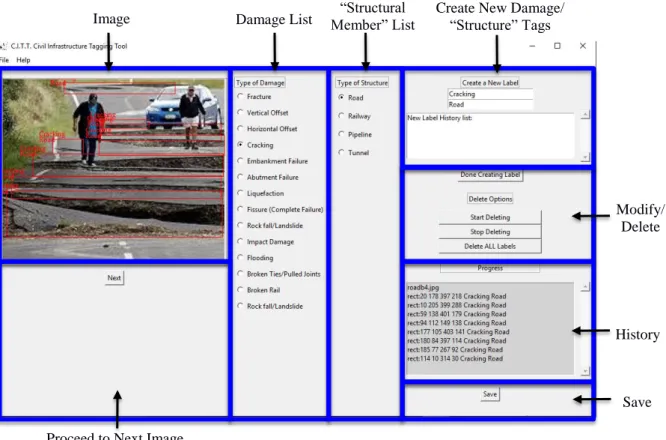
reconnaissance work. One issue with existing image repositories, other than the lack of annotations, is that naming conventions between engineers are inconsistent. The image tagging tool provides a simple mechanism for a group of experts to share common damage and structural member list that appear as pre-set/static radio buttons, leading to greater annotation consistency and improved searchability of resulting image databases. Aside from speed and consistency, the tool also has flexibility of creating user-generated damage-structure tags and modifying/deleting existing tags such that an expert can easily revise the work of a skilled novice. Figure 1 presents the graphical user interface (GUI) of the image tagging tool for civil infrastructure damage; the image on the upper left is being tagged for “cracking-road” where a red bounding box is draw around each occurrence of the target damage-structure type.
Figure 1. Civil infrastructure image tagging module (blue boxes and labels added for clarity).
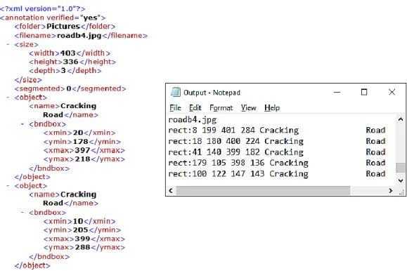
One of the most important capabilities of the tool is that it outputs a PASCAL VOC (Everingham et al. 2015) annotation (.xml) file for each tagged image which is compatible with most deep learning frameworks (Goodfellow et al. 2016), including TensorFlow (Abadi et al. 2016); additionally, a common text (.txt) file is generated. Samples of both output file types, shown in Figure 2, record the image name as well as each occurrence of a damage-structure pair and location of associated bounding box in the image. These output file formats allow data scientists and engineers rapid parsing abilities to easily conduct robust statistical analyses of the damage-structure pairs occurring in a large image set for an individual or multiple earthquake.
3. DESCRIPTION OF DEEP LEARNING ALGORITHM
In recent years, computer vision algorithms based in DL have made automatic image classification an easier task since these approaches embed feature extraction (recognizing patterns in an image) within a learning pipeline (Goodfellow et al. 2016). These algorithms are loosely based on biological neural systems where an individual neuron does a simple operation and sends the output signal to the rest of the neurons; a single neuron does very little, but in a network they can perform very complex tasks.
Image Damage List Member” List “Structural Create New Damage/ “Structure” Tags
Modify/ Delete
History
Save
4
Figure 2. Portions of sample output files from image tagging tool: (left) PASCAL VOC, .xml; (right) text, .txt.
3.1 General Description of Neural Network Structure
To elaborate, each neuron is simulated as a simple software function and these neurons are connected together in groups create a layer, as shown in Figure 3. The number of neurons per layer is chosen by the data scientist, except for the input layer which depends on the size of the input image. For example, if the input image is 32 x 32 pixels then the input layer will contain 1024 (=322) neurons. Training a neural network (NN) entails adjusting the weight of each neuron in a layer such that the classification errors in the “ground truth” training set are minimized. For the example with a 32 x 32 pixel image and a neural network with 10 layers at 512 neurons each, a single training step will require the NN to learn almost three million weights as calculated per:
Wtotal = Ninput + L ∙ Nlayer + Noutput = (32 ∙ 32) + (32 ∙ 32) ∙ 512 + (10-1) ∙ 512 ∙ 512+ 512 ∙ 2 =
~ 2.8 million weights (1)
where Wtotal is the total number of weights to learn; Ninput and Noutput are the number of neurons in the input and output layers, respectively; and Nlayer is the number of neurons in each of the other layers.
As illustrated in Figure 3, the input pixel value, Xi, is multiplied by the learned weight for each corresponding neuron, Wij , and added to all other neuron outputs from a layer, Σ Xi ∙ Wij. The summation of all neuron outputs including bias, Bi, (y-intercept of the activation function, F(x)) is calculated for a layer. If this value exceeds the lower bound set for the activation function, in the form F(x) = max (0, F(x)), then the output in that layer pass to the next level. This is the process that enables each interconnected layer to learn a simple higher-level feature extraction and by connecting many layers it is possible to identify entire objects in an image.
5
Figure 3. Simplified representation of deep learning: (Left) Neuron (Right) Layers.
3.2 Stages for Implementing Neural Network
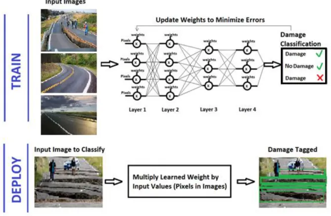
Implementation of neural networks (NN) requires two stages. The first is training the NN on a set of “ground truth” images which contain data known to be correctly classified. Once the NN has been trained and the optimal weight for each of the neurons determined, the second stage is to deploy the NN such that the learned weights from the training stage are utilized to classify a new image. Figure 4 illustrates the two stages of the neural network workflow specifically as it pertains to classification of damage in civil infrastructure images.
Figure 4. Neural network workflow.
6
(ii) results in algorithms that are easier to train and optimize, and (iii) produces high-quality results for an array of visual recognition tasks. In fact, Russakovsky et al. (2015) demonstrated that ResNet achieves an outstanding 3.57% error rate on the ImageNet set which contains millions of images and thousands of categories (performance that exceeds human error rates of 5-10%). The TensorFlow framework was selected to implement ResNet as it is relatively easy to program and scales to multiple GPUs to accelerate training time. Figure 5 illustrates the steps the authors used to develop the DL using ResNet and TensorFlow to classify civil infrastructure damage.
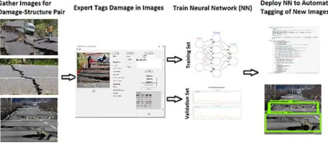
Figure 5. Deep learning steps for damage classification of above-ground civil infrastructure.
The following descriptions provide further detail on the steps described in Figure 5:
1.Gather images for a damage-structure pair: There is no specific number of input images necessary to train a DL algorithm; however, generally more is better. The research team has been able to train to 80% accuracy using a set of ≥ 100 images, and 90-93% with ≥ 200 images (though these results are also dependent on the difficulty of identifying patterns for a damage-structure pair).
2.Expert tags damage in images: The authors created a software tool described in Behrouzi & Pantoja (2018) that an expert or skilled novice engineer can utilize to place a bounding box around each instance of the target damage-structure pair in the collected input images. This software stores the bounding box location and associated labels in the PASCAL VOC output format (Everingham et al. 2015) which is a compatible input for most DL frameworks. The manually tagged images form the “ground truth” image set for training/validating the DL algorithm.
3.Train neural network (NN):
Divide the tagged images: The full set of tagged input images is divided into two groups. The training set serves as input to the algorithm in the learning process, and the validation set is used to test that the algorithm is learning correctly. In their image classification tasks related to buildings and civil infrastructure damage detection, the authors generally use a randomized ~ 75% / 25% split of the tagged input images to develop the training and validation sets.
Train: Each neuron is initialized to a given weight, and training iterations consist of: (i) calculating error/loss functions based on the NN’s performance in classifying validation
images, (ii) modifying neuron weights to correct for error determined in (i) via an optimization approach like gradient descent, and (iii) re-training using the new weights. Training terminates when the DL algorithm achieves an adequate validation accuracy.
7
only a small time offset to ensure the algorithm is learning at a desired pace.
4. Deploy NN to automate tagging of new images: Once an adequate validation accuracy for classifying a specific damage-structure pair is achieved, the DL algorithm consisting of the weights for each neuron can be saved to a Jupyter notebook (similar to Pantoja & Behrouzi 2017). This trained NN, for a given damage-structure pair, can now be deployed by other users to identify the same features on new sets of images.
4. RESULTS
To test the DL implementation, two different sets of damage-structure pairs were used as “ground truth” images. The first was of roadways with cracking of different severities; and the second was of railway tracks that exhibited horizontal offset/lateral offset.
4.1 Classification of Roadway with Cracking
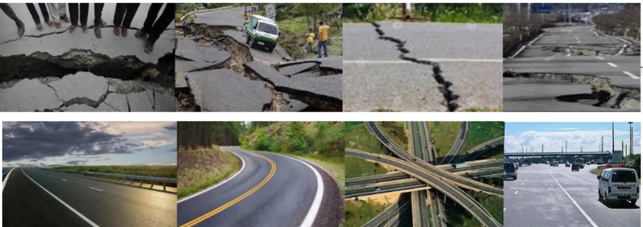
Figure 6 presents a subset of the input images to train the algorithm for the general classification category of roadway with cracking. The input image set includes cracking oriented in longitudinal and transverse directions with respect to the road. Additionally damage in these images ranges from minor to severe, including: (i) cracking – relatively insignificant roadway rupture such that the integrity of road is not compromised and transportation can continue without repair, (ii) fracture – more significant than cracking and typically requires repair before normal road traffic can resume, and (iii) fissure – complete failure of roadway resulting in the transportation artery being completely impassible which requires long-term closure and replacement.
Figure 7 shows the output generated by the trained algorithm, it can be seen that the algorithm can tag multiple instance of the damage in a single photo. The algorithm is able to achieve an accuracy of around 92% against the image validation set. For this classification task of roadway cracking, the authors are releasing the input image set and validation scripts with neuron weights from the trained NN as a Jupyter notebook (Pérez & Granger 2007) via GitHub (Pantoja & Behrouzi 2017). Other users can input test images to the specified directory and review their results.
Figure 6. Input images for roadways: (top) cracking, (bottom) no cracking.
8
Figure 7. Output images from deep learning classifier for the set of images from Figure 6. Note: If the algorithm does not detect damage, the original image will remain unchanged as seen with images of no cracking.
4.2 Classification of Railway with Horizontal Offset/Lateral Translation
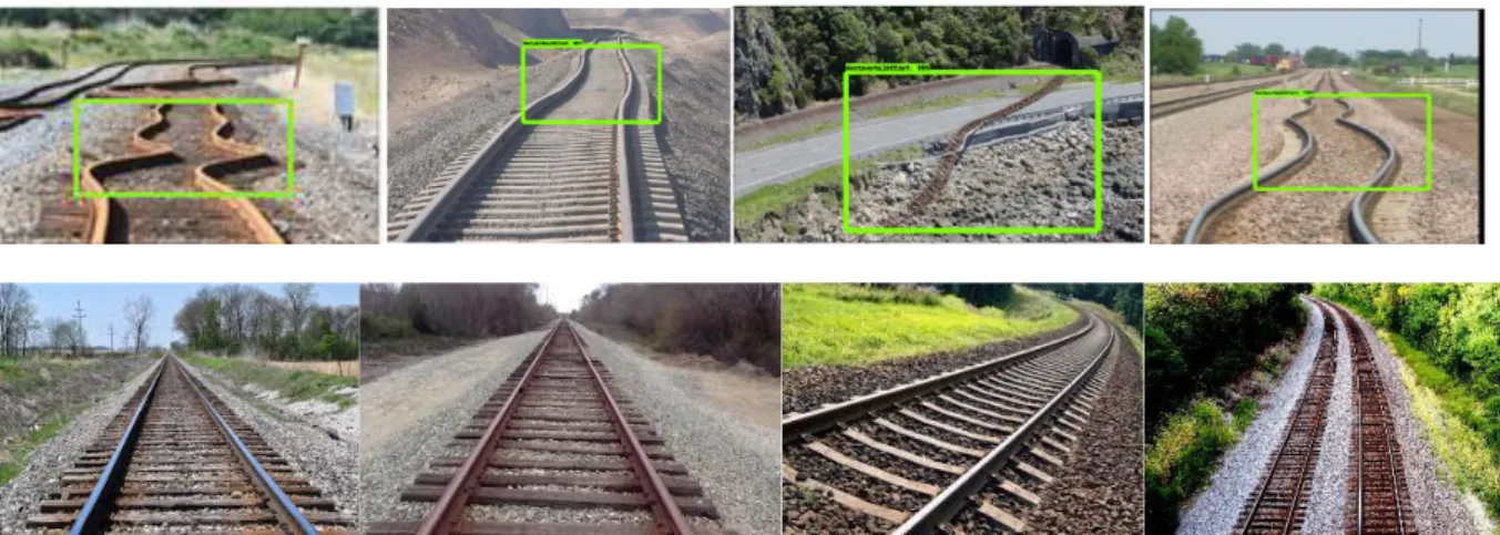
Figure 8 presents a subset of the input images used to validate the algorithm for railway tracks due to horizontal offset/lateral translation. For this damage type only 100 training images were utilized as it is less prevalent than damage types like roadway cracking (which had around 150 training images). Another challenge is filtering out rail track buckling due to temperature differences, train-track interaction, and weakened track conditions; causes which are not related to railway horizontal offset resulting from ground rupture or motion during an earthquake.
Figure 9 shows current output from the algorithm. Results on this set are promising with 80% accuracy. As more post-earthquake photographs of rail track horizontal offset are identified and tagged for training of the NN, accuracy will improve.
Figure 8. Input images for railways: (top) horizontal offset, (bottom) no horizontal offset.
Future work on this damage type includes collecting/tagging more training images to improve the NN accuracy prior to publicly release via GitHub. Additionally, it does not yet appear that the algorithm consistently tags multiple instances of the target damage in a single image; seen in several of the examples shown in Figure 9. Efforts will be made to address these items.
9
Figure 9. Output images from deep learning classifier for the set of images from Figure 8. Note: If the algorithm does not detect damage, the original image will remain unchanged as seen with images of no horizontal offset.
5. CONCLUSIONS AND FUTURE WORK
The objective of the research work described in this paper was to create a tool based on computer vision to automatically annotate post-earthquake civil infrastructure damage images, which will facilitate the inspection/evaluation process conducted by professional structural engineers and assist with the rapid deployment of emergency and repair teams in the aftermath of a major seismic event. The results show that a DL solution yields a high level of accuracy ≥80% even with limited image training sets between 100-150 images. The authors expect as more images become available for training the NN, there will be improvements in both the general classification task and location assignment of bounding boxes for each occurrence of target damage in an image. The research team also seeks to classify more complex tags, including multiple distinct tags in a single image (i.e. roadway cracking and railway horizontal offset in the same photograph).
In the future, the intention is to use 500-1000 images tagged by 2+ experts for each damage-structure pair that is commonly observed in civil infrastructure after an earthquake. This will include combinations of damage and structure types indicated in the lists from the image tagging tool GUI (Figure 1). The authors plan to release tagged images as an open source database for other experts to build and add upon as well as the DL algorithm used to classify this combination of damage-structure pairs so other researchers can replicate the results and/or expand for their own data sets.
The future of visual recognition in civil infrastructure should be based on computer vision. This technology is not to serve as a substitute for expert structural engineers, but to facilitate their job by presenting experts with a refined set of images on which to concentrate their efforts in much the same way that DL algorithms are helping radiologists to analyze MRI images for cancer detection by pre-selecting areas of interest (Esteva et al. 2017).
6. ACKNOWLEDGMENTS
The work described is this paper was supported by California Polytechnic State University – San Luis Obispo via the CPConnect and Research, Scholarly, and Creative Activities (RCSA) Grant Programs. Thanks also to Caleb Azevedo, Jack Bergquist, and Anugrah Gupta assisted with image collection.
7. REFERENCES
10
Levenberg J, Monga R, Moore S, Murray DG, Steiner B, Tucker P, Vasudevan V, Warden P, Wicke M, Yu Y, Zheng X (2016). TensorFlow: a system for large-scale machine learning. 12th USENIX Conference on Operating Systems Design and Implementation: 265-283.
Barrington L, Ghosh S, Greene M, Har-Noy S, Berger J, Gill S, Yu-Min Lin A, Huyck C (2011). Crowdsourcing earthquake damage assessment using remote sensing imagery. Annals of Geophysics, 54 (6): 680-687.
Behrouzi A, Pantoja M (2018). Photo Tagging Tool for Rapid and Detailed Post-Earthquake Structural Damage Identification. Proceedings of the 11th National Conference in Earthquake Engineering (11NCEE).
Brilakis I, German S, and Zhu Z (2011). Visual pattern recognition models for remote sensing of civil infrastructure. Journal of Computing in Civil Engineering, (25) 5, 388-393.
Esteva A, Kuprel B, Novoa RA, Ko J, Swetter SM, Blau HM, Thrun S (2017). Dermatologist-level classification of skin cancer with deep neural networks. Nature. (542) 7639: 115-118.
Everingham M, Eslami SMA, Van Gool L, Williams CKI, Winn J, Zisserman A (2015). The PASCAL Visual Object Classes Challenge: a Retrospective. Int’l Journal of Computer Vision, 111(1), 98-136.
Feng C, Liu MY, Kao CC, Lee TY (2017). Deep active learning for civil infrastructure defect detection classification. ASCE International Workshop on Computing in Civil Engineering.
Goodfellow I, Bengio Y, Courville A. Deep learning. MIT Press 2016. www.deeplearningbook.org.
He Z, Zhang X, Ren X, Sun J (2016). Deep residual learning for image recognition. IEEE Conference on Computer Vision and Pattern Recognition.
Jahanshahi M (2017). Deep learning for condition assessment of civil infrastructure systems. GPU Technology Conference.
Koch C, Doycheva K, Kasireddy V, Akinci B, Fieguth P (2015). A review on computer vision based defect detection and condition assessment of concrete and asphalt civil infrastructure. Journal of Advanced Engineering Informatics, (29) 2, 196-210.
Krizhevsky A, Sutskever I, Hinton G (2012). ImageNet classification with deep convolutional neural networks. Advances in neural information processing systems.
Patterson B, Leone G, Pantoja M, Behrouzi A (2018). Deep learning for automated image classification of seismic damage to build infrastructure. Proceedings of the 11NCEE.
Pantoja M, Behrouzi A (2017). ImageTagVER. Github. https://github.com/mpantoja314/ImageTagVER.
Pérez F, Granger BE (2007). IPython: A System for Interactive Scientific Computing, Computing in Science and Engineering, (9)3: 21-29.
Russakovsky O, Deng J, Su H, Krause J, Satheesh S, Ma S, Huang Z, Karpathy A, Khosla A, Bernstein M, Berg A, Fei-Fei L (2015). ImageNet large scale visual recognition challenge. Int’l Journal of Computer Vision, (115) 3, 211-252.
Stanford Urban Resilience Initiative (2017). Remote assessment of damage using the crowd: Capitalizing on the crowd after an earthquake. Stanford Urban Resilience Initiative. http://urbanresilience.stanford.edu/rad-crowd/
Yeum, CM (2016). Computer vision-based structural assessment exploiting large volumes of images. PhD Thesis, Purdue University.