An Inverse Problem Method for Gas Temperature Estimation in Partially Filled Rotating Cylinders

An Inverse Problem Method for Gas Temperature

Estimation in Partially Filled Rotating Cylinders

M.M. Heydari

_{and B. Farhanieh}

The objective of this article is to study gas temperature estimation in a partially lled rotating cylinder. From the measured temperatures on the shell, an inverse analysis is presented for estimating the gas temperature in an arbitrary cross-section of the aforementioned system. A nite-volume method is employed to solve the direct problem. By minimizing the objective function, a hybrid eective algorithm, which contains a local optimization algorithm, is adopted to estimate the unknown parameter. The measured data are simulated by adding random errors to the exact solution. The eects of measurement errors on the accuracy of the inverse analysis are investigated. Two optimization algorithms are used in determination of the gas temperature. The conjugate gradient method is found to be better than the Levenberg-Marquardt method, since the former produces more accurate results for the same measurement errors. A good agreement between the exact value and the estimated result has been observed for both algorithms.

INTRODUCTION

In recent years, much eort has been devoted to study inverse analysis in many design and manufac-turing problems, especially when direct measurement of surface conditions is not possible. The analysis of Inverse Heat Conduction Problems (IHCP) has numerous applications in various branches of science and engineering.

Inverse heat transfer problems, in contrast to di-rect heat transfer problems, belong to a set of problems that become unstable under small changes in the initial data. In fact, well and ill-posed problems of mathemat-ical physics are distinguished and diculties associated with the solution of IHTP should also be recognized. Mathematically, inverse heat transfer problems belong to a class called ill-posed [1-7], whereas standard heat transfer problems are well-posed.

Conventionally, the inverse problem includes two phases: The process of analysis and the process of optimization. In the analysis process, the unknown pa-rameters or functions are assumed and the results of the problem are solved directly through either analytical methods [8], such as Laplace transform [9], or

numeri-1. Center of Excellence in Energy Conversion, Department of Mechanical Engineering, Sharif University of Technol-ogy, P.O. Box 11155-9567, Tehran, Iran.

*. To whom correspondence should be addressed. E-mail: [email protected]

cal methods, such as nite dierence and nite element methods [10-14] and dynamic programming [15]. In the optimization process, an optimizer, such as in the Levenberge-Marquardt method, conjugated gradient method and steepest descent method [16,17], is used to guide the exploring points systematically to search for a new set of guess parameters. These new data could be substituted for unknown parameters in the analysis process.

Several numerical and experimental studies have been performed for the estimation of unknown point heat sources and boundary conditions in cylindrical coordinate systems using IHCPs [18-22]. The investiga-tion of thermal behavior in hollow cylinders employing an inverse methodology has also been reported [23-25]. A literature survey of the available work, points out the lack of investigation of thermal behavior in a rotating cylindrical container using an inverse method-ology.

A partially lled rotating cylinder is a funda-mental physical concept that can be used in mathe-matical modeling of many industrial processes, such as drying, heating (cooling), calcining, separating, mixing, reducing, roasting, sterilizing, food making and metallurgical processes and in the sintering of a variety of materials [26-36].

In this study, a parameter estimation of quasi-steady conduction-convection heat problems has been undertaken using a numerical inverse analysis solver based on nite volume formulation in cylindrical

coor-dinates. The gas temperature in an arbitrary cross-section of a rotating cylinder has been determined using an inverse algorithm. The eectiveness of the inverse algorithm was assessed using a sensitivity study. For assurance as to the eectiveness of the developed algorithm, dierent experimental data were examined. To discuss the correlation between measuring locations and the accuracy of the results, two types of measuring location were considered. Two inverse heat techniques were used for hot gas estimation in an arbitrary cross-section of an innite long rotating cylinder. For damping instabilities in the inverse analysis procedure, iterative parameter estimation techniques were consid-ered.

PROBLEM FORMULATION

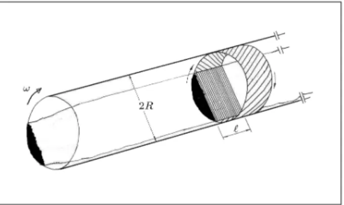
The considered partially lled rotating cylinder is presented, schematically, in Figure 1. The geometrical properties are 4.5 m for the internal radius, 6 m for the external radius and 2.25 m for the bed depth. The rotational speed of the hollow cylinder is 1.5 rad/s and the used material properties in the direct model are given in Table 1.

GOVERNING EQUATION

In the cylinder, the bed (plug ow) region rotates as a rigid body about the hollow cylinder axis. A cylindrical coordinate system is used in this region, as well as for the wall itself. Energy conservation for any cylindrical control volume in the plug ow region and the wall (refractory lining), as shown in Figure 2, requires the

Figure 1. 3-D schematic presentation of partially lled rotating cylinder.

Table 1. Relevant physical properties. Property Charge Wall k (W/m/_{K) 0.692 0.4}

(kg/m3_{) 1680 1334}

Cp(J/kg/K) 1298 1100-1300

Figure 2. Two-dimensional cross-section model.

following: 1 r

@ @r

kir@T_@r

+_r1_2@@

ki@T_@

+_@z@

ki@T_@z

= iCpiu_r@@T ; i = w; p; (1)

where; u= r!:

In order to predict temperature distribution in the considered long rotating cylinder, the following as-sumptions were made:

1. Due to high length-to-diameter ratio eects in the system, the conduction heat transfer in the longitudinal direction is negligible, i.e. @Ti

@z = 0:0,

2. The charge behavior at the cross-section is as in rolling bed mode,

3. The hydrodynamic behavior of the charge at the bed is as plug ow,

4. Both the hollow cylinder wall and the bed are taken to be relatively gray [37-40],

5. The owing gas (freeboard gas) is taken to be relatively gray,

6. There are no radial temperature gradients in the freeboard gas, so that either phase could be char-acterized by a unique temperature at a given cross-section of the hollow cylinder.

Applying appropriate simplications to the phys-ical model, the governing partial dierential equation (Equation 1) reduces as follows [28]:

1 r

@ @r

kir@T_@r

+_r1_2@@

ki@T_@

According to Figure 2, the following boundary condi-tions could be used:

a. At the exposed inner wall for 0 2 0:

r = Ri;

0 2 0:

k@T_@r = (hCg!ew+ hRg;p!ew)(Tg Tew): (3)

b. At the charge surface (exposed solid surface) for

2 0 0;

r = R();

2 0 0:

k@T_@r = (hCg!p+ hRg;ew!p)(Tg Tp): (4)

The value of Tg in Equations 3 and 4 should be

obtained by inverse analysis. c. Initial conditions for ;

Ri T icr Ro:

T (r; = 0) = T (r; = 2)

@T (r;=0)

@r = @T (r;=2)@r :

(5) The radiative heat transfer coecients, i.e. hRg;p!ew; hRg;w!p, can be calculated from a

multi-zone radiation model [40,41].

The convective heat transfer coecient be-tween the owing hot gas and the exposed wall can be determined from the following correla-tion [32,40,42,43]:

hCg!ew = 0:036

kg

DRe0:8Pr0:33

D L

_0:055

: (6)

The convective heat transfer coecient from the owing hot gas to the bed (plug ow) can be de-termined from the following correlation [28,32,40]:

hCg!p = 0:4G0:62g : (7)

d. At the outer hollow cylinder surface (shell) for 0 2;

r = Ro;

0 2 :

k@T_@r = (hCsh!1+ hRsh!1)(Tsh T1): (8)

The radiative heat transfer coecient at the outer shell, hRsh!1, could be evaluated using:

hRsh!1=

"sh(T4sh T14)

(Tsh T1) : (9)

The natural convection, (Re2

D< GrD), heat

trans-fer between the shell surface of the cylinder and the surroundings could be evaluated by [44]:

Nu = hsh_kD 1 = 0:6

+ 0:386Ra1=6

[1+(0:559=Pr)9=16_]8=27;

10 4_<Ra<1012_{; (10)}

where:

Ra = Pr GrD: (11)

INVERSE ANALYSIS CONCEPT

As stated in the introduction, in practical problems, it may be dicult to obtain some of the unknown pa-rameters and functions through direct measurement, as the desired positions of the sensors cannot be accessed. However, they can be obtained through inverse heat conduction analyses. Inverse analysis is a discipline that provides tools for the ecient use of the sensor values of measured temperature data in estimation of the structure of the mathematical models and, also, unknown parameters, functions and the initial and boundary conditions appearing in mathematical mod-els [1-14]. For the parameter or function estimation, error is dened by the dierence between the measured and estimated or computed temperatures (e = Te

Tc_{). Minimization of this error is the main goal of}

inverse analysis. One of the minimization strategies is to apply the standard least squares method.

The solution of this inverse problem for the esti-mation of N unknown parameters, Pj, j = 1; ; N,

is based on minimization of the ordinary least squares norm, given by [24]:

S(P ) = [Te _Tc_{(P )][T}e _Tc_{(P )]}T_{: (12)}

The estimated temperature, Tc

i(P ) = T (P; xi), is

obtained from the solution of the direct problem at the measurement location, xi, which corresponds with the

experimental temperature, Te_{. To minimize the least}

squares norm given by Equation 12, the derivative of S(P), with respect to each of the unknown parameters, P = [p1; p2; ; pn], should be equated to zero. Such

a necessary condition for the minimization of S(P) can be represented in matrix notation by equating

the gradient of S(P), with respect to the vector of parameter P to zero, that is:

rS(P) = 2 "

@TcT

(P ) @P

#

[Te _Tc_{(P )] = 0: (13)}

Sensitivity Analysis

The solution of inverse problems and the accuracy of the estimated parameters and functions are directly related to the sensitivity of the measurements to the errors in input data, due to the location of the sensors and frequency of oscillations. The sensitivity matrix is determined by dierentiating Equation 12, with respect to the vector of the unknown parameters or functions as follows:

J(P ) = @Tc

T

(P )

@P : (14)

The elements of the sensitivity matrix are called sen-sitivity coecients. A sensen-sitivity coecient is very important because it indicates the magnitude of a change in the temperature, due to perturbations in the value of parameters or functions.

Using the denition of sensitivity from Equa-tion 14, the sensitivity coecient distribuEqua-tion can be determined by dierentiating governing Equation 2, with respect to the vector of the unknown parameters or functions, P , as follows:

1 r

@ @r

kir@J_@r

+_r1_2@@

ki@J_@

= iCpi!@J_@; i = w; p: (15)

The initial and boundary conditions read as follows: r = Rin;

0 2 0:

k@J_@r = (hCg!ew+ hRg;p!ew); (16)

r = R();

2 0 0:

k@J_@r = (hCg!p+ hRg;ew!p); (17)

Ri T ic r Ro : J(r; = 0) = J(r; 2);

@J(r; = 0)

@r =

@J(r; = 2)

@r : (18)

Inverse Analysis Methods

In inverse analysis methods, unknown quantities can be estimated by minimizing the least squares, Equa-tion 12. These methods, based on estimaEqua-tion of an unknown quantity, can be divided into two groups; parameter estimation and function estimation. There are several parameter estimation methods available for inverse analysis to treat the ill-posed nature of inverse problems, e.g., the least squares method modied by the addition of a regularization term, and the use of a conjugate gradient method, where the regularization is inherently built into the iterative procedure [1,2,5,6]. There are some powerful techniques for solving inverse heat transfer problems. These techniques are as follows [24]:

1. Levenberg-Marquard method for parameter estima-tion,

2. Conjugate Gradient method for parameter estima-tion,

3. Conjugate Gradient method with an adjoint prob-lem for parameter estimation,

4. Conjugate Gradient method with an adjoint prob-lem for function estimation.

The parameter estimation approaches are, in general, nonlinear and the number of the unknown parameters is strongly limited [7]. However, in the parameter esti-mation methods, there is a priori inforesti-mation regarding the functional forms of the unknown parameters and their locations. It is also generally assumed that the number of these parameters/functions and their coecients are known.

However, for cases with no priori information of the functional forms, one must use the function estimation methods of the inverse analysis, such as the adjoint conjugate gradient method and the func-tion specicafunc-tion method. The solufunc-tion of funcfunc-tion estimation problems is highly sensitive to noise in the measured data. Even if data were measured exactly, the inverse function estimation problems would be dicult. However, for function estimation, if some information is available on the functional form of the unknown function, the inverse problem of estimating this function is reduced to estimating a nite number of parameters.

The Levenberg-Marquardt and the conjugate gra-dient methods, based on minimization of the objective function, are the two iterative algorithms used in this study for parameter estimations. These inverse heat conduction methods for estimating unknown parame-ters and functions are conducted for certain sequential items, i.e. solution of the direct problem, solution of the inverse problem and a convergence criterion. These methods can be suitably arranged in iterative proce-dures. In this research, both Levenberg-Marquardt

and Conjugate Gradient methods are used for gas temperature estimation.

Levenberg-Marquardt Method

In this parameter estimation method, for the minimiza-tion of Equaminimiza-tion 12, its gradient, with respect to the vector of the unknown parameters, must be equated to zero.

Using the denition of the sensitivity matrix, Equation 13 could be written as:

2JT_{(P )[T}e _Tc_{(P )] = 0: (19)}

The solution of Equation 19 for nonlinear estimation problems requires an iterative procedure, which is obtained by linearizing the vector of the estimated temperatures, Tc

i(P), with a Taylor series expansion

around the current solution, Pk_{, at iteration k. Such a}

linearization is given by:

Tc_{(P ) = T}c_(Pk_{) + J}k_{(P P}k_{): (20)}

Equation 20 is substituted into Equation 19 and the resulting expression is rearranged to yield the following iterative procedure, in order to obtain the vector of the unknown parameters, P. Inverse problems are generally very ill conditioned, especially near the initial guess used for the unknown parameters. Levenberg-Marquardt alleviates such diculties by utilizing an iterative procedure in the following form [24,25]:

Pk+1_=Pk_+[(Jk₎T_Jk₊kk_] 1_(Jk₎T_[Te _Tc_(Pk_)];

(21) where k _{is a diagonal matrix used for alleviating}

the ill-conditioned problem and k _{is a positive scalar}

called the damping factor. Conjugate Gradient Method

The conjugate gradient method is a powerful itera-tive parameter or function-estimation algorithm for the solution of linear and nonlinear inverse problems. In this method, the following principle relations are considered [24,25].

In the conjugate gradient method, the minimiza-tion procedure is performed by using the following iteration:

Pk+1_{= P}k k_dk_{: (22)}

At each iteration step, a suitable step size, k_{, is taken}

along the direction of descent in order to minimize the objective function.

The direction of the descent is obtained as a linear combination of the negative gradient direction at the current iteration, with the direction of descent of the previous iteration, which is as follows:

dk _{= rS(P}k_{) +} k_dk 1_{; (23)}

where:

k ₌ N

P

j=1f[rS(P k_)]

j[rS(Pk) rS(Pk 1)]jg N

P

j=1[rS(P k_)]2

j

;

0_{= 0: (24)}

The gradient direction vector is determined as: rS(Pk_{) = 2(J}k₎T_[Te _Tc_(Pk_{)]: (25)}

Temperature vector, T (Pk k_dk_{), can be linearized}

with a Taylor series expansion and, then, the mini-mization, with respect to k_{, is performed to yield the}

following expression for the search step size:

k₌ N

P

j=1[J

k_dk_]T_[Tc_(Pk_{) T}e_] N

P

j=1f[J k_]T_dk_g2

: (26)

Convergence Criterion

The above-mentioned iterative algorithms need a crite-rion to stop the iterative procedure of the solution. The following condition is used for terminating the iterative process:

S(Pk+1_{) < "} 1;

(Jk₎T_{[Y T (P}k)] < " 2;

Pk+1 _Pk < "

3: (27)

The solution of inverse problems using an iterative algorithm may become well posed if the convergence criterion is used to stop the iterative procedure. NUMERICAL ANALYSIS

Direct Method Algorithm

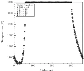
The nite volume-method is employed to solve the bed-wall governing equation for the cross-section of the partially lled rotating cylinder. Rectangular grids with cylindrical control volumes are used in both the plug ow (charge) and the wall regions. The grid independency study, as shown in Figure 3, on the mesh in the solution domain, indicates that the 131 45 grids in and r directions, respectively, are sucient to produce grid independent results. The generated mesh for the computational domain is presented in Figure 4.

Figure 3. The eect of dierent grid sizes on radial temperature distribution.

Figure 4. Computational grid for partially lled rotating cylinder (cross section).

Inverse Method Algorithm

A quasi-steady-state heat conduction-convection in-verse problem was developed for the partially lled rotating cylinder. As shown in Figure 5, the gas tem perature in the arbitrary cross-section, Tgas, could

be estimated using the inverse problem method. For estimation of the unknown parameter, the objective function, S(Pk_{), should be optimized. This objective}

function is produced, based on the measured and com-putational temperature dierences at the shell surface of the rotating hollow cylinder. Due to employment of the L.M.M. algorithm, Equations 20 or 21 should be computed iteratively. To perform the iteration, according to C.G.M, the direction of the descent vector, dk_{, in Equation 23 and the step size,} k_{, in Equation 26}

Figure 5. Layout of cross-section model with thermocouple arrangement shown.

require computation. For both optimization algo-rithms, the iteration producer is continued until one of the criteria introduced in Equation 27 is satised. RESULTS

The properly developed inverse algorithm should lead to the correct value of the parameter in question. The eectiveness of the inverse algorithm can be assessed using the sensitivity study. To assess the eectiveness of the developed algorithm, dierent experimental data with 0%, 1% and 5% error were examined. To discuss the correlation between the measuring locations and the accuracy of the results, two types of measuring location were considered. The rst location is the entire perimeter of the shell surface of the rotating cylinder's cross-section and the second location is the bedside zone of the shell. For each location, three sets of thermocouple arrangement, as shown in Fig-ure 5, were considered. Both Levenberg-Marquardt and Conjugate-Gradient optimization algorithms were applied for each thermocouple arrangement.

Sensitivity Analysis

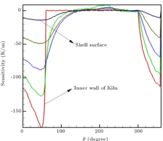
Sensitivity coecients are, in some sense, the key to the success of the estimation procedures of the parameter and verify the inuence of the measured parameters (measured temperatures). The sensitivity variations for gas temperature estimation are computed in four dierent layers of the rotating cylinder wall and are presented in Figure 6. As seen from this result, the sensitivity coecient for gas temperature estimation at the inner wall is better, with respect to the outer wall (shell), for all thermocouple arrangements. In addition, the sensitivity coecient in the bedside zone of the cross-section (at inner or outer walls) is considerable

Figure 6. Sensitivity study for gas temperature estimation in dierent wall layers of cross section.

with respect to other zones. Therefore, it is expected that computational analysis based on covered wall actual temperature data, converges faster compared with computational analysis based on other isoclines experimental data.

Experimental Data

In order to simulate the measured temperature, Tmeasure, (by imaginary thermocouples) realistic noises

are introduced to contaminate the theoretical tem-perature, Texact, computed from the solution of the

direct problem. The results involving the random mea-surement errors, the normally distributed uncorrelated errors with non-zero mean and constant standard devi-ation were assumed. Thus, the measured temperature, Tmeasure, could be expressed as follows:

Tmeasure = Texact(1 + ); (28)

where Texactis the solution of the direct problem with

the exact gas temperature, 1600_{K, is the standard}

deviation of the measurement and is the random variable, which is within 2:576 2:576 for 99.43% condence bound [16,22-25]. The produced measuring data for shell and bedside zones of a cylinder with 0%, 1% and 5% errors are shown in Figures 7 and 8, respectively.

Numerical Test Case 1

As shown in Figure 5, 27, 33 and 44 thermocouples, in turn, are arranged at the perimeter shell surface at an arbitrary cross-section of the rotating cylinder. The results of this inverse study for C.G.M and L.M.M algorithms are shown in Figures 9 and 10, respectively. The options (a), (b) and (c) are related to the 26,

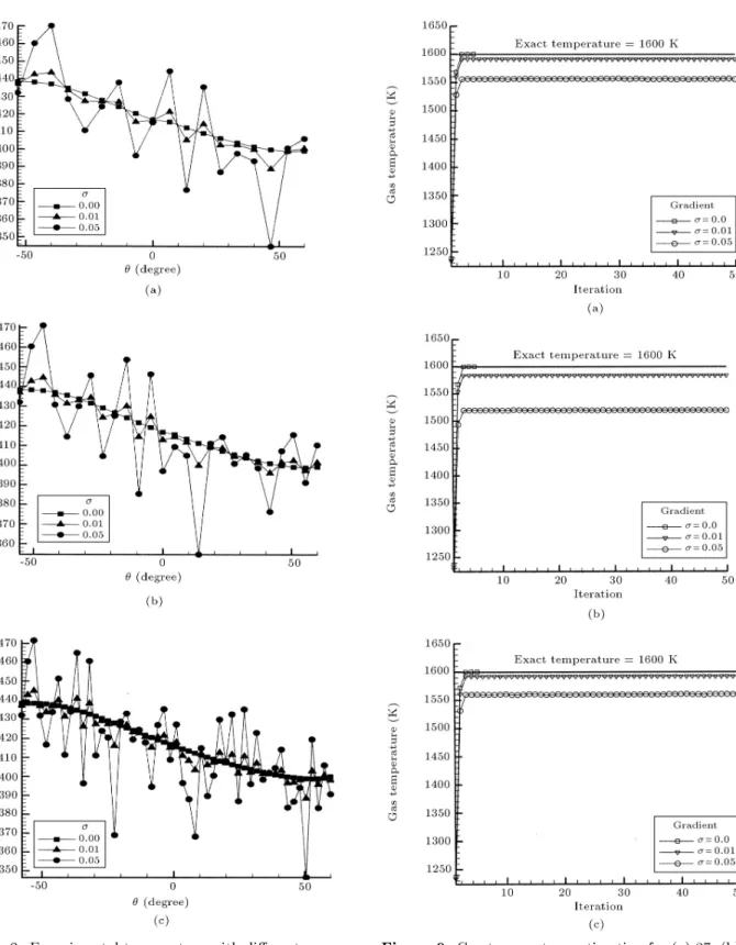
Figure 7. Experimental temperature with dierent error for (a) 27, (b) 33 and (c) 44 thermocouples arrangement on the shell.

33 and 44 thermocouples, respectively. These gures illustrate that the estimated results have excellent approximations with the exact value of the gas tem-perature when the measurement error is not considered to be = 0:0. In addition, the estimated results

Figure 8. Experimental temperature with dierent error for (a) 18, (b) 26 and (c) 51 thermocouples arrangement on the bedside zone.

are in good agreement with the aforementioned exact value, even when the measurement error, = 0:01, is considered. These results show that the accuracy of the gas temperature increases as the number of thermocouples are increased to an optimum value.

Figure 9. Gas temperature estimation for (a) 27, (b) 33 and (c) 44 thermocouples on the shell based on C.G.M. algorithm.

For example, as shown in Figures 9 and 10, it is obvious that an optimum value for the thermocouples arrangement is 33. Also, the results obtained by using C.G.M are better than the results obtained by using L.M.M. regarding accuracy and CPU time.

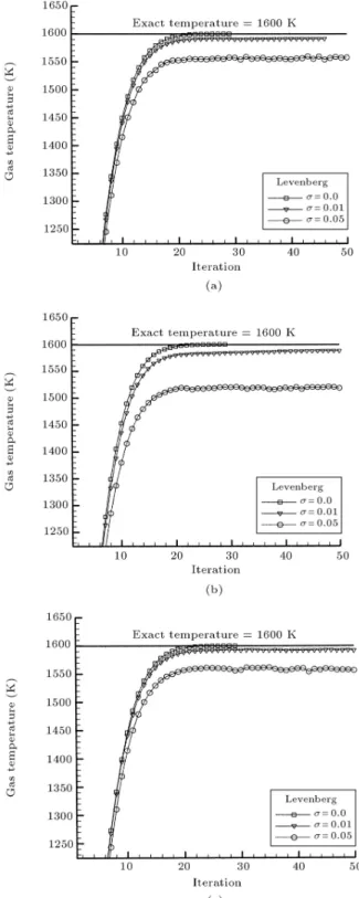
Figure 10. Gas temperature estimation for (a) 27, (b) 33 and (c) 44 thermocouples on the shell based on L.M.M. algorithm.

Numerical Test Case 2

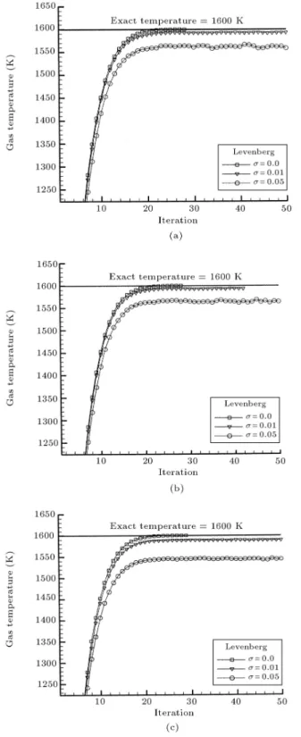
18, 26 and 51 thermocouples, in turn, are arranged at an arbitrary cross-section on the bedside zone of the shell of the rotating cylinder. The results of

Figure 11. Gas temperature estimation for (a) 18, (b) 26 and (c) 51 thermocouples on the bedside zone based on C.G.M. algorithm.

this test case are presented in Figures 11 and 12. These gures illustrate that the estimated results have excellent approximations with the exact value of the gas temperature when the measurement error is not considered to be = 0:0. Also, the estimated results

Figure 12. Gas temperature estimation for (a) 18, (b) 26 and (c) 51 thermocouples on the bedside zone based on L.M.M. algorithm.

are in good agreement with the aforementioned exact value, even when the measurement error, = 0:01, is considered. In addition, these results show that the accuracy of the gas temperature increases as the number of thermocouples is increased to an optimum

value. As shown in Figures 11 and 12, it is obvious that an optimum value for thermocouple arrangement is 10. Also, the results obtained using C.G.M are better than the results obtained using L.M.M. regarding accuracy and CPU time.

CONCLUSION

In this paper, a method for estimating the hot gas temperature in a partially lled rotating cylinder is developed. This parameter is estimated by an ex-perimental temperature via an inverse method. Two examples were used to show the robustness of the proposed method. The Levenberg-Marquardt method and the conjugate gradient method with a nite vol-ume approach were successfully applied for solution of the inverse problem, in order to determine the gas temperature, by utilizing temperature readings at the shell of the rotating cylinder. The results show that the C.G.M does not require an accurate initial guess of unknown quantities, needs very short CPU time and requires fewer sensors, when compared with the L-MM, in performing the inverse calculations.

From the results, it appears that, by using the proposed method, without measurement error, the exact solution (exact value for gas temperature) can be found, even with only few measurement points. When measurement errors are included, in order to enhance stability and accuracy, temperature data requires more measuring points on the shell surface. Furthermore, fewer measurement points on the bedside of the shell surface, with respect to the whole surface of the shell, may be used to obtain accurate results.

Consequently, the results conrm that the pro-posed inverse method is eective and ecient for gas temperature estimation in a partially lled rotating cylinder.

NOMENCLATURE

A area

Cp specic heat

D hollow cylinder diameter d direction of descent vector

E emissive power

G mass ow rate of gas

h convection coecient

J sensitivity matrix

J radiosity

k conductivity

M number of measuring Temperature

N number of unknowns

P estimated parameter

Pr Prandtl number

r polar coordinate

Ri inner radius of hollow cylinder

Ro outer radius of hollow cylinder

Re Reynolds number

Ra Rayleigh number

S square root of errors

T temperature

T average temperature

T ic bed depth

absorptivity

search step size (descent parameter)

conjugate coecient

! hollow cylinder angular velocity " emissivity

"1; "2; "3 tolerance for convergence of the

iterative inverse methods

r reectivity

angular coordinate

density

measurement error

s Stephan-Boltzman constant

the probability or random value

dynamic viscosity

0 ll percent

dimensionless temperature

S gradient of S

Superscript

c computational

e experimental

k iteration step

T transpose

average value Subscript

a; 1 ambient

p plug ow (bed)

cw covered wall

ew exposed wall

exact exact value

g gas

i measured parameter index

j unknown parameter index

measure measurement value

over overall

sh shell

w wall

REFERENCES

1. Hadamard, J., Lectures on: Cauchy's Problem in Linear Dierential Equations, Yale University Press, New Haven, CT (1923).

2. Tikhonov, A.N. and Arsenin, V.Y., Solution of Ill Posed Problems, Winston & Sons, Washington, DC (1977).

3. Backus, G. and Gilbert, P. \Numerical applications of a formalism for geophysical inverse problems", Geophys J. Roy. Astron, 13, pp 247-276 (1967). 4. Beck, J.V. and Arnold, K.J., Parameter Estimation:

in Engineering Estimation, John Wiley & Sons Pub. (1977).

5. Beck, J.V. and Blackwell, B., Inverse Heat Conduc-tion: Ill-Posed Problems, Wiley, New York (1985). 6. Beck, J.V., Blackwell, B. and St. Clair, C.R., Inverse

Heat Conduction-Ill Posed Problem, Wiley, New York (1985).

7. Mozorov, V.A. and Stressin, M. \Regularization Method for Ill-posed problem", CRC Press Boca Ra-ton, FL (1993).

8. Burggraf, O.R. \An exact solution of the inverse problem in heat conduction theory and applications", ASME Journal of Heat Transfer, 84, pp 373-382 (1964).

9. Arledge R.G. and Haji-Sheykh, A. \An iterative ap-proach to the solution of inverse conduction heat problem", Numerical Heat Transfer, 1, pp 365-376 (1978).

10. Fidelle, T.P. and Zinsemeister, G.E. \A semi-discrete approximate solution of the inverse problem of tran-sient heat conduction", A.S.M.E. Paper No. 68-WA/HT-26 (1968).

11. Beck, J.V. \Nonlinear estimation applied to the non-linear inverse heat conduction problem", International Journal of Heat and Mass Transfer, 13, pp 703-716 (1970).

12. D'Souza, N. \Numerical solution of one-dimensional inverse transient heat conduction by nite dierence method", A.S.M.E. Paper No. 75-WA/HT-81 (1975). 13. Krutz, G.W., Schoenhals, R.J. and Hore, P.S. \Appli-cation of the nite element method to the inverse heat conduction problem", Numerical Heat Transfer, 1, pp 489-498 (1978).

14. Beck, J.V., Litkouhi, B. and St Clair, Jr, C.R., \Ecient sequential solution of the nonlinear heat conduction problem", Numerical Heat Transfer, 5, pp 272-286 (1982).

15. Beck, J.V. and Litkouhi, B. \Ecient sequential solution of the nonlinear heat conduction problem", Numerical Heat Transfer B, 27, pp 291-307 (1995). 16. Necati Ozisik, M., Inverse Heat Transfer, Taylor &

Francis 29 West 35th Street, New York, NY (2000). 17. Liu, G.R. and Han, X., Computational Inverse

Tech-niques in Nondestructive Evaluation, CRC PRESS LLC (2003).

18. Su, J. and Silva Neto, A.J. \Two-dimensional inverse heat conduction problem of source strength estimation in cylindrical rods", Appl. Math. Modeling, 25, pp 861-872 (2001).

19. Raynaud, M. \Some comments on the sensitivity to sensor location of inverse heat conduction problems using Beck's method", Int. J. Heat Mass Transfer, 29(5), pp 815-817 (1986).

20. Bartsch, G., Schroeder-Richter, D. and Huang, X.C. \Quenching experiments with a circular test section of medium thermal capacity under forced convection of water", Int. J. Heat Mass Transfer, 37(5), pp 803-818 (1994).

21. Nguyen, K.T. and Bendada, A. \An inverse approach for the prediction of the temperature evolution during induction heating of a semi-solid casting billet", Mod-elling Simul. Mater. Sci. Eng., 8, pp 857-870 (2000). 22. Lin, J.H., Chen, C.K. and Yang, Y.T. \Inverse

esti-mation of the thermal boundary behavior of a heated cylinder normal to a laminar air stream", Int. J. Heat Mass Transfer, 43(21), pp 3991-4001 (2000).

23. Lin, J.H., Chen, C.K. and Yang, Y.T. \An inverse method for simultaneous estimation of the center and surface thermal behavior of a heated cylinder normal to a turbulent air stream", Int. J. Heat Mass Transfer, 124, pp 601-608 (2002).

24. Yang, Y.T., Hsu, P.T. and Chen, C.K. \A three-dimensional inverse heat conduction problem approach for estimating the heat ux and surface temperature of a hollow cylinder", Journal of Physics D: Applied Physics, 30, pp 1326-1333 (1997).

25. Hsu, P.T., Yang, Y.T. and Chen, C.K. \Simultane-ously estimating the initial and boundary conditions in a two-dimensional hollow cylinder", International Journal of Heat and Mass Transfer, 41(1), pp 219-227 (1998).

26. Brimacombe, J.K. and Watkinson, A.P. \Heat transfer in direct-red rotary Kiln, I- Pilot plant and experi-mentation, II- Heat ow results and their interpreta-tion", Met. Trans. B., l9B, pp 201-219 (1978). 27. Barr, P.V., Brimacombe, J.K. and Watkinson, A.P.

\A heat transfer model for the rotary kiln, Part I. Pilot hollow cylinder trials, Part II. Development of cross-section mode", Met. Trans. B., 20B, pp 391-419 (1989).

28. Boateng, A.A. \Rotary kiln transport phenomena; study of the bed motion and heat transfer", PhD. Dissertation, The University of British Columbia, Van-couver (1993).

29. Marcio, A. and Learndo, S. \Modeling and simulation of petroleum coke calcinations in rotary kiln", FUEL, 80, pp 1-15 (Jan. 2001).

30. Baker, C.G.J. \Cascading rotary dryers", Advances in Drying, 2, pp 1-51 (1983).

31. Maciej, S. and Mohamed, M. \Modeling of rotating drum dryer for sugar", AVH Association - 11th Sym-posium - Reims (March 2004).

32. Kadir, B.B. \Flow phenomena in horizontal axially rotated partially lled cylinder", Thesis for Degree of Doctor of Philosophy, Dalhousie University (1998). 33. Carslow, H.S. and Jager, J.C., Conduction of Heat in

Solid, Clarendon Press, Oxford, GBR (1973).

34. Cannon, J.N. \Heat transfer to a uid owing inside a pipe rotating about its longitudinal axis", J. Heat Transfer, 91, pp 135-139 (1969).

35. Gavish, J., Chadwick, R.S. and Gutnger, C. \Viscous ow in a partially lled rotating horizontal cylinder", Israel J. Techno, 1(16), pp 264-272 (1978).

36. Heydari, M.M. and Farhanieh, B. \Bed depth esti-mation in rotary kiln by inverse problem method", International Conference on Numerical Analysis and Applied Mathematics, WILEY (2005).

37. Gorog, J.P., Brimacombe, J.K. and Adams, T.N. \Radiative heat transfer in rotary kiln", Metallurgical Transaction B, 12B, pp 55-70 (March 1981).

38. Gorog, J.P., Brimacombe, J.K. and Adams, T.N. \Re-generative heat transfer in rotary kiln", Metallurgical Transaction B, 13B, pp 153-163 (June 1982). 39. Gorog, J.P., Brimacombe, J.K. and Adams, T.N.

\Heat transfer from ames in rotary kiln", Metallurgi-cal Transaction B, 14B, pp 411-424 (Sept. 1982). 40. Ghoshdastidar, P.S. and Anandan Unni, V.K. \Heat

transfer in the non-reacting zone of a cement rotary kiln", ASME Journal of Engineering for Industry, 118, pp 169-172 (1996).

41. Siegel, R. and Howell, J.R., Thermal Radiation Heat Transfer, McGraw-Hill, New York (1981).

42. Tscheng, S.C. and Watkinson, A.P. \Convective heat transfer in a rotary kiln", The Canadian J. of Chem. Eng., 57 (1979).

43. Kreith, F. and Black, W.Z., Basic Heat Transfer, Harper & Row, New York, NY (1980).

44. Ozisik M.N., Heat Transfer, 2nd Ed Montreal, Mc-Graw Hill (1985).