Vol 6, No 10 (2015)

Available online throug

ISSN 2229 – 5046

INFLUENCE OF TEMPERATURE-DEPENDENT VISCOSITY ON THE MHD COUETTE FLOW

OF DUSTY COUPLE STRESS FLUID WITH HEAT TRANSFER

V. P. RATHOD

_{, SYEDA RASHEEDA PARVEEN*}

1

_{Department of Studies and Research in Mathematics,}

Gulbarga University, Gulbarga-585 106, Karnataka, India.

(Received On: 28-09-15; Revised & Accepted On: 28-10-15)

ABSTRACT

T

Key-words: couette flow, magnetohydrodynamics, heat transfer, dusty couple stress parameter.

INTRODUCTION

The flow of dusty couple stress fluid and electrically conducting fluid through a channel in the presence of transverse magnetic field has important application in many devices such as magnetohydrodynamic (MHD) power generators. MHD pumps, accelerators, aerodynamics heating electrostatic, precipitation polymer technology, petroleum industry, purification of Molten metal’s from non-metallic inclusions and fluid droplets-sprays.

The flows of couple stress fluids have many practical application in modern technology and industries, led various researchers to attempt diverse flow problems related to several Non-Newtonian fluids one such fluid that has attracted the attention of numerous researchers in fluid mechanics during the last five decades in the theory of couple stress fluid proposed by Stokes [1]. The concept of couple stress arises due to the way in which the mechanical interactions in the fluid medium are modeled. Singh and Pathak [2] have discussed unsteady flow of a dusty viscous fluid through a uniform pipe with sector of a circle as cross-section, and Pulsatile flow of blood with micro-organism through a uniform pipe with sector of a circle as cross-section in the presence of transverse magnetic field has been investigated by Rathod and Parveen [3]. Also unsteady flow of a dusty magnetic conducting couple stress fluid through a pipe and the flow of a conducting fluid in a circular pipe has been investigated by many authors Gudiraju et.al, [4]. Dube and Sharma [5] and Ritter and Peddieson [6] have reported solutions for unsteady dusty gas flow in a circular pipe in the absence of a magnetic field and particle phase viscous stress. Rathod et.al, [7] have reported solution for couette flow of a conducting dusty visco-elastic fluid through two flat plate under the influence of transverse magnetic field. Rathod and Rasheeda [8] investigated unsteady flow of a dusty magnetic conducting couple stress fluid through a circular pipe and Rathod and Rasheeda [9] have studied by unsteady MHD couette flow with heat transfer of a couple stress fluid under exponential decaying pressure gradient. The hydrodynamic flow of dusty fluid was studied by a number of authors. Later the influence of the magnetic field on the flow of electrically conducting dusty fluid was studied [10, 11, 12]. Most of these studies are based on constant physical properties. More accurate prediction for the flow and heat transfer can be achieved by taking into account the variation of these properties especially the variation of the fluid viscosity with temperature [13]. Attia and Kotb [14] studied the steady MHD fully developed flow and heat transfer between two parallel plates with temperature – dependent viscosity.

Corresponding Author: Syeda Rasheeda Parveen*

_{Department of Studies and Research in Mathematics,}

In the present work, the effect of variable viscosity on the unsteady laminar flow of on electrically conducting viscous, couple stress, dusty fluid and heat transfer between parallel non-conducting porous plates are studied. The fluid is flowing between two electrically insulating infinite plates maintained at two constant but different temperatures. An external uniform magnetic fields applied perpendicular to the plates. The upper plate is moving with a uniform velocity while the lower is kept stationary. The magnetic Reynolds number is assumed small so that the induced magnetic field is neglected. The fluid is acted upon by a constant pressure gradient and viscosity is assumed to vary exponentially with temperature. The flow and temperature distributions of both the fluid and dust particle are governed by the couple set of the momentum and energy equations. The Joule and viscous dissipation terms in the energy equation are taken into consideration. The governing couple non lineal partial differential equations are solved using transformation method, the effects of the external uniform magnetic field, couple stress parameter and the temperature – dependent viscosity on the time development of both the velocity and temperature distributions are discussed.

DESCRIPTION OF THE PROBLEM

The dusty couple stress fluid is assumed to be flowing between two infinite horizontal plates located at the y=± h planes. The dusty particles are assumed to be uniformly distributed throughout the fluid. The two plates are assumed to be electrically non-conducting and kept at two constant temperature T1 for the lower plates and T2 for the upper plates

with T2 > T1. The upper plate is moving with a uniform velocity vo while the lower is kept stationary. A constant

pressure gradient is applied in the x-direction and the parallel plates are assumed to be porous and subjected to a uniform suction from above and injection from below. Thus y-component of the velocity is constant and denoted by

vo. A uniform magnetic field Bo is applied in the +ve y-direction. By assuming a very small magnetic Reynolds number

the induced magnetic field is neglected [15]. The fluid motion starts from rest at t=o, and the no-slip condition at the plates implies that the fluid and dust particles velocities have neither a z–nor an x–component at y=±h. The initial temperature of the fluid and dust particle are assumed to be equal to T1 and the fluid viscosity is assumed to vary

exponentially with temperature. Since the plates are infinite in the x – and y – directions. The physical variable are invariant in these directions. The flow of the fluid is governed by the Navier-stokes equation [16].

𝛠𝛠𝜕𝜕𝜕𝜕_{𝜕𝜕𝜕𝜕} + ϱ𝛾𝛾0𝜕𝜕𝜕𝜕_{𝜕𝜕𝜕𝜕} = - 𝑑𝑑𝑑𝑑_{𝑑𝑑𝑑𝑑} + _{𝑑𝑑𝜕𝜕}𝑑𝑑 �𝜇𝜇𝜕𝜕𝜕𝜕_{𝜕𝜕𝜕𝜕}� - 𝐵𝐵𝑜𝑜2 u - 𝜂𝜂∇2(∆2u) - kN(u-up) (1)

Where 𝛠𝛠 is density of the clean fluid, 𝜇𝜇 is the viscosity of the clean fluid, u is the velocity of the fluid. 𝜕𝜕_𝑑𝑑 is the velocity of the dust particle. 𝜂𝜂 is the parameter of couple stress fluid, 𝝈𝝈 is the electric conductivity p is the pressure acting on the fluid, N is the number of the dust particles per unit volume and k is the constant. The first four terms in the right hand side are, the pressure gradient, viscosity and Lorentz force, Parameter of couple stress fluid, respectively.

The last term represent the force term due to the relative motion between fluid and dust particles. It is assumed that the Reynold number of the relative velocity is small. In such a case the force between dust and fluid is proportional to the relative velocity [17]. The motion of the dust particle is governed by Newton’s Second law [17].

mp

𝜕𝜕𝜕𝜕𝑑𝑑

𝜕𝜕𝜕𝜕 = kN (u-up). (2)

Where mp is the average mass of dust particles, the initial and boundary conditions on the velocity fields are

respectively, given by t=o, u=up=o (3)

for t>o, the no-slip condition at the plates implies that

y = - h, u=o, y=h, u=uo (4)

Heat transfer takes place from the upper hot plates towards the lower cold plate by conduction through the fluid. Also, there is a heat generation due to both the Joule and viscous dissipations. The dust particles gain heat energy from the fluid by conduction through their spherical surface. Two energy equations are required which describe the temperature distributions for both the fluid and dust particles are respectively, given by [11].

𝛠𝛠c 𝜕𝜕𝜕𝜕

𝜕𝜕𝜕𝜕 + ϱ c 𝛾𝛾0 𝜕𝜕𝜕𝜕 𝜕𝜕𝜕𝜕 = k

𝜕𝜕2_𝜕𝜕

𝜕𝜕𝜕𝜕2 + 𝜇𝜇�

𝜕𝜕𝜕𝜕 𝜕𝜕𝜕𝜕�

2

+ 𝜎𝜎𝐵𝐵_𝑜𝑜2𝜕𝜕2 + 𝜚𝜚𝑑𝑑𝐶𝐶𝑠𝑠

𝛾𝛾𝜕𝜕 (Tp – T) (5)

𝜕𝜕𝜕𝜕𝑑𝑑

𝜕𝜕𝜕𝜕 = −1

𝛾𝛾𝜕𝜕 (Tp – T) (6)

Where T is the temperature of the fluid, Tp is the temperature of the particles. c is the specific heat capacity of the fluid

at constant pressure, cs is the specific heat capacity of the particle, k is the thermal conductivity of the fluid. 𝛾𝛾_𝜕𝜕 is the

temperature relaxation time �−3𝑃𝑃𝑟𝑟𝛾𝛾𝑑𝑑𝐶𝐶𝑠𝑠

2𝐶𝐶 �. 𝛾𝛾𝑑𝑑 is the velocity relaxation time � −2𝜌𝜌𝑠𝑠𝐷𝐷2

9𝜇𝜇 �, 𝜌𝜌s is the material density of dust

particles ( 3𝜌𝜌𝑑𝑑

t ≤ o: T = Tp = o.

t > o, y = - h, T = T1

t > o, y = h: T = T2 (7)

The viscosity of the fluid is assumed to depend on temperature and is defined as μ = 𝜇𝜇₀ 𝑓𝑓(T) for practical reasons which are shown to be suitable for most kinds of fluids [16, 17]. The viscosity is assumed to vary exponentially with temperature.

The formation f(T) takes the form [16, 17], f(T) = 𝑒𝑒𝑏𝑏(𝜕𝜕−𝜕𝜕1), where the parameter be has the dimension of f[T]-1 and such that at T = T1, f(T1) = 1 and then μ = 𝜇𝜇𝑜𝑜 this means that 𝜇𝜇𝑜𝑜 is the viscosity coefficient at T = T1 the parameter a

may take the values for liquids such as water, benzene, or crude oil. In some gases like air, helium, or methane a1, it

may be negative, that is, the coefficient viscosity increases with temperature [16, 17].

The temperature variations with in a convective blow give rise to variations in the properties of the fluid in the density and viscosity, for example. An analysis including the full effects of there is a complicated that some approximations become essential. The equations are commonly used in a form known as the Boussineq approximation. In Boussineq approximation variations of all fluid properties other than the density are ignored completely variations of the density are ignored except insofar as they give rise to gravitational force [12], therefore, a buoyancy force term may be included in the Navier Stokes equation which equals ∝ 𝝔𝝔∆𝙏𝙏, where ∝ is the coefficient of expansion of the fluid. Such a buoyancy term may be neglected on the basis of either ∆𝙏𝙏 small,that is, T2 – T1 is small, or small ∝ which is a

reasonable approximation for liquid and perfect gasses [12].

The problem is simplified by writing the equations in the dimensional form. We define the following non-dimensional quantities.

(𝑑𝑑�,𝜕𝜕) = (x�,y�)

ℎ , t = 𝜕𝜕/𝜕𝜕𝑜𝑜

𝜚𝜚ℎ2, 𝑃𝑃� = _{𝜚𝜚𝜕𝜕}𝑃𝑃_𝑜𝑜2, 𝜆𝜆 = −𝑑𝑑𝑃𝑃�_{𝑑𝑑𝑑𝑑�}, (𝜕𝜕�,𝑣𝑣�) = (𝜕𝜕_/,𝑣𝑣_𝜕𝜕)𝜚𝜚ℎ

𝑜𝑜 , (𝜕𝜕�𝑑𝑑, 𝑣𝑣�p) =

(�𝜕𝜕𝑑𝑑,𝑣𝑣�𝑑𝑑,)𝜚𝜚ℎ

𝜚𝜚𝜕𝜕𝑜𝑜 , 𝜕𝜕� =

𝜕𝜕−𝜕𝜕1

𝜕𝜕2−𝜕𝜕1 , 𝜕𝜕�p =

Tp−𝜕𝜕1

𝜕𝜕2−𝜕𝜕1

f(T) = 𝑒𝑒−𝑏𝑏(𝜕𝜕2−𝜕𝜕1)𝜕𝜕 _{= 𝑒𝑒}−𝑎𝑎𝜕𝜕_{, a is the viscosity variation parameter;}

𝐻𝐻𝑎𝑎2 = 𝜎𝜎𝐵𝐵𝑜𝑜

2_ℎ2

𝜇𝜇𝑜𝑜 , Ha is the Hartmann number, R=𝐾𝐾𝑁𝑁ℎ2

𝜇𝜇𝑜𝑜 , is the particle concentration parameter. G = 𝑚𝑚𝑑𝑑𝜕𝜕𝑜𝑜

ℎ𝑘𝑘 is the particle mass parameter.

s = 𝒱𝒱𝑜𝑜

𝜕𝜕𝑜𝑜 is the suction parameter, 𝑃𝑃𝑟𝑟 =

𝜇𝜇𝑜𝑜𝑜𝑜

𝑘𝑘 is the prandtl number

Ec =

𝜇𝜇𝑜𝑜2

ℎ2_{𝑜𝑜𝜚𝜚}2_𝑒𝑒𝑏𝑏(𝜕𝜕2−𝜕𝜕1) is the Eckert number. Lo =

𝜚𝜚ℎ2

𝜇𝜇𝑜𝑜𝒱𝒱𝜕𝜕 is the temperature relaxation time parameter.

In terms of the above non-dimensional quantities the velocity and energy equations read.

𝜕𝜕𝜕𝜕 𝜕𝜕𝜕𝜕 + s

𝜕𝜕𝜕𝜕

𝜕𝜕𝜕𝜕 = s + 𝑓𝑓(T) 𝜕𝜕2𝜕𝜕

𝜕𝜕𝜕𝜕2 + 𝜕𝜕𝜕𝜕_{𝜕𝜕𝜕𝜕}𝜕𝜕𝑓𝑓_{𝜕𝜕𝜕𝜕}(𝜕𝜕) - _𝛼𝛼�12𝜕𝜕 4_𝜕𝜕

𝜕𝜕𝜕𝜕4 - 𝐻𝐻𝑎𝑎2u – R(u-up) (8)

G 𝜕𝜕𝜕𝜕𝑑𝑑

𝜕𝜕𝜕𝜕 = u – up (9)

𝜕𝜕𝜕𝜕 𝜕𝜕𝜕𝜕 + s

𝜕𝜕𝜕𝜕 𝜕𝜕𝜕𝜕 =

1 𝑃𝑃𝑟𝑟

𝜕𝜕2𝜕𝜕

𝜕𝜕𝜕𝜕2 + Ec 𝑓𝑓 (T) �𝜕𝜕𝜕𝜕_{𝜕𝜕𝜕𝜕}�

2

+ Ec 𝐻𝐻_𝑎𝑎2u2 + 2𝑅𝑅

3𝑃𝑃𝑟𝑟 (Tp – T), (10)

𝜕𝜕𝜕𝜕𝑑𝑑

𝜕𝜕𝜕𝜕 = - Lo (Tp – T), (11)

t ≤ o: T = Tp = o.

t > o, y = - 1; T = o = Tp, (12)

t > o y = 1: T = 1 = Tp,

Equations (8), (9), (10) and (11) represent a system of coupled and nonlinear partial differential equations which are solved by using transformation method (Cosine and Hankle transformation).

u = 4𝜆𝜆

∝𝐺𝐺�

(−1)m

n ∞

𝑚𝑚=𝑜𝑜 1 𝑑𝑑2

2 ∝ �1−

(∝2𝑒𝑒∝1𝜕𝜕−∝1𝑒𝑒∝2𝜕𝜕)

�𝑑𝑑12− 4𝑑𝑑2

�� Jo(yℇi)

ℇiJ1(ℇi)

∞

𝑖𝑖=1 cos (2𝑚𝑚+1)⊼𝜕𝜕

2∝ (13)

up = �

4𝜆𝜆

∝𝐺𝐺 �

(−1)m

n ∞

𝑚𝑚=𝑜𝑜 1 𝑑𝑑2 �

Jo(yℇi)

J1(ℇi)

∞

𝑖𝑖=1 cos

(2𝑚𝑚+1)⊼𝜕𝜕 2∝ � .

��1_𝐺𝐺− 1� − 1

�𝑑𝑑12− 4𝜕𝜕2

(∝2(𝑒𝑒∝1𝜕𝜕−𝑒𝑒 −1

𝐺𝐺 𝜕𝜕) ∝1+ 1_𝐺𝐺 −

∝1(𝑒𝑒∝2𝜕𝜕−𝑒𝑒 −1

𝐺𝐺 𝜕𝜕)

T = (𝛽𝛽2𝑆𝑆𝜕𝜕=𝑜𝑜)𝑒𝑒𝛽𝛽1𝜕𝜕

𝛽𝛽2−𝛽𝛽1 +

(Ś𝜕𝜕=𝑜𝑜−𝛽𝛽1𝑆𝑆𝜕𝜕=𝑜𝑜)𝑒𝑒𝛽𝛽2𝜕𝜕

𝛽𝛽2−𝛽𝛽1 + S (15)

Tp = (𝛽𝛽₂𝑆𝑆_{𝜕𝜕=𝑜𝑜}− Ś_{𝜕𝜕=𝑜𝑜})(𝑒𝑒

𝛽𝛽1𝜕𝜕_−𝑒𝑒−𝐿𝐿𝑜𝑜𝜕𝜕₎

𝛽𝛽1+𝐿𝐿𝑜𝑜 + (Ś𝜕𝜕=𝑜𝑜− 𝛽𝛽1𝑆𝑆𝜕𝜕=𝑜𝑜)

(𝑒𝑒𝛽𝛽2𝜕𝜕_−𝑒𝑒−𝐿𝐿𝑜𝑜𝜕𝜕₎

𝛽𝛽2+𝐿𝐿𝑜𝑜 +𝜕𝜕₅ 𝜕𝜕4�1−𝑒𝑒−𝐿𝐿𝑜𝑜𝜕𝜕�

𝐿𝐿𝑜𝑜 +

1

𝑑𝑑₁2_{−4𝑑𝑑2} (𝜕𝜕4+2𝜕𝜕3∝1) ∝2(𝑒𝑒

2∝1𝜕𝜕_−𝑒𝑒−𝐿𝐿𝑜𝑜𝜕𝜕₎

�4∝₁2_{+2∝1𝜕𝜕1𝜕𝜕2�(2∝1+𝐿𝐿𝑜𝑜)}

+(𝜕𝜕4+2𝜕𝜕3)∝3∝1(𝑒𝑒2∝1𝜕𝜕−𝑒𝑒−𝐿𝐿𝑜𝑜𝜕𝜕)

�4∝22+2∝2𝜕𝜕1+𝜕𝜕2�(2∝2+𝐿𝐿𝑜𝑜) -

2∝1∝2(𝜕𝜕4+(∝1∝2)𝜕𝜕3)(𝑒𝑒(∝1 ∝2)−𝑒𝑒−𝐿𝐿𝑜𝑜𝜕𝜕)

((∝1∝2)2+((∝1∝2)𝜕𝜕1+𝜕𝜕2)((∝1∝2+𝐿𝐿𝑜𝑜)

−2 �𝑑𝑑12− 4𝑑𝑑2

�(𝜕𝜕4+∝1𝜕𝜕3)∝2 (𝑒𝑒∝1𝜕𝜕−𝑒𝑒−𝐿𝐿𝑜𝑜𝜕𝜕)

�∝12+∝1𝜕𝜕1+𝜕𝜕2�(∝1+𝐿𝐿𝑜𝑜) −

(𝜕𝜕4+∝2𝜕𝜕3)∝1 (𝑒𝑒∝2𝜕𝜕−𝑒𝑒−𝐿𝐿𝑜𝑜𝜕𝜕)

�∝22+∝1𝜕𝜕1+𝜕𝜕2�(∝2+𝐿𝐿𝑜𝑜) � (16)

Where X1 = S + 𝑓𝑓(T) +

1

𝛼𝛼�2 + 𝐻𝐻𝑎𝑎2 + R +

1

𝐺𝐺, X2 =

𝑆𝑆 𝐺𝐺 -

𝜆𝜆 𝐺𝐺 +

𝑓𝑓(𝜕𝜕) 𝐺𝐺 -

1 𝛼𝛼�2_𝐺𝐺 -

𝐻𝐻𝑎𝑎2

𝐺𝐺

Y1 = S + _𝑃𝑃1

𝑟𝑟 + L, Y2 =

𝐿𝐿

𝑃𝑃𝑟𝑟 + LS, Y3 = EcK + 2Ec𝐻𝐻𝑎𝑎

2_{, Y}

4 = LEcK + LEc𝐻𝐻_𝑎𝑎2, ∝1 = 1₂ �−𝑑𝑑1+ �𝑑𝑑12−4𝑑𝑑2�, ∝2 = 1₂ �−𝑑𝑑2− �𝑑𝑑12−4𝑑𝑑2�

𝛽𝛽1 = 1₂ �−𝜕𝜕1+ �𝜕𝜕12−4𝜕𝜕2�, 𝛽𝛽2 = 1₂ �−𝜕𝜕1− �𝜕𝜕12−4𝜕𝜕2�

Y5 = �_∝𝐺𝐺4𝜆𝜆 � (−1) m

n x2

∞

𝑚𝑚=𝑜𝑜 �

Jo(yℇi)

J1(ℇi)

∞

𝑖𝑖=1 cos

(2𝑚𝑚+1)⊼𝜕𝜕 2∝ �

2

S = Y5 Y4+ _(𝑑𝑑 1 1

2_{−4𝜕𝜕2)}�(𝜕𝜕4+2𝜕𝜕3)∝2𝑒𝑒 2∝1𝜕𝜕

�4∝₁2_{+2∝1𝜕𝜕1+𝜕𝜕2�}+ (𝜕𝜕4+2𝜕𝜕3∝2)∝1𝑒𝑒 2∝2𝜕𝜕

�4∝₂2_{+2∝2𝜕𝜕1+𝜕𝜕2�} −2∝1∝2(𝜕𝜕4+(∝1+𝜕𝜕2)𝜕𝜕3) 𝑒𝑒 (∝1+∝2)𝜕𝜕

((∝1+∝2)2(∝1∝2)𝜕𝜕1+𝜕𝜕2) �

- 2

�𝑑𝑑12−4𝑑𝑑2

�(𝜕𝜕4+∝1𝜕𝜕3)∝2𝑒𝑒∝1𝜕𝜕

�∝₁2_{+∝1𝜕𝜕1+𝜕𝜕2�} + (𝜕𝜕4+∝2𝜕𝜕3)∝1𝑒𝑒 ∝2𝜕𝜕

�∝₂2_{−∝2𝜕𝜕1+𝜕𝜕2�} �

Computations have been made for R = 0.5, G = 0.8, = 5, Pr = 1, Ec = 0.2, and Lo = 0.7. Plotted the graph for different

values of couple stress parameter, suction parameter, Hartman, decaying parameter and time by using “Mathematica”.

RESULT AND DISCUSSION

The exponential dependence of the viscosity on temperature results in decomposing the viscous force term in the momentum equation in to two terms. The variation of these resulting terms with the viscosity variation a and their relative magnitude have an important effect on the flow and temperature fields in the absence or presence of applied uniform magnitude field.

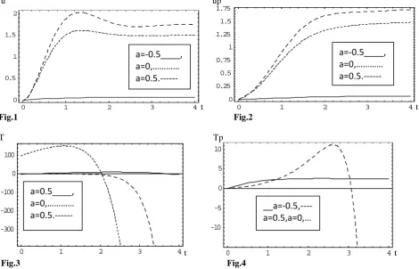
Figures 1 and 2 indicate the variation of the velocities u and up at the center of the channel (y=o) and q=0.1 (couple

stress parameter) with time for different values of the viscosity variation parameter a and for Ha = 0 and s=0. the figures

shows that increasing 𝑎𝑎 increasing the velocity and the time required to approach the steady state, the effect of the parameter 𝑎𝑎 on the steady state time is more pronounced for the values of a than for negative values. It is clear, u reaches the steady state faster than up. This is because the fluid velocity is the source for the dust particle velocity. It is also shows that the influence of 𝑎𝑎 on u and up are negligible for some time and then increases as the time develops.

Figures 3 and 4 present the variations of the temperature T and Tp at the center of the channel y = o and q = 0.1 with

time for different values of the viscosity variation parameter𝑎𝑎 a for Ha = 0 and s = 0. The Figures show that increasing 𝑎𝑎 increasing the temperature and the steady state times.Increasing the positive values of 𝑎𝑎 increase the temperature, for small times but decrease, it y as time develops, thus increasing a and is longer for T them for Tp, as Tp always follows T

it is noticed that the steady state values of T coincide with corresponding state, state values of Tp and the time required

for T to read steady state, which depends on a, is longer than Tp.

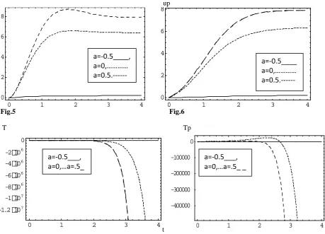
The application of the uniform magnetic field adds on resistive term to momentum equation and Joule dissipation term to energy equation. Figures 5 and 6 present the influence of the viscosity variation parameter a on the evolution of both the velocity u and up at the centre of the channel for Ha = 1 and s =0, respectively. The magnetic field results in a

reduction in the velocity and steady state time for all values of a due to damping effect.

Figures 7 and 8 present the influence of the viscosity variation parameter a on the violation of the temperature T and Tp

at the center of channel, respectively for Ha= 1, and s = 0. Increasing the magnetic field decreases the temperatures for

Figures 9 and 10 present the variation of the velocity u and up at the centre of the channel y = o with time for different

values of the viscosity variation parameter a and for Ha = 0, s = 1 and q = 0.1. It is clear that the suction velocity

decreases both u and up and their steady state times as a result of pumping of the fluid from the lower half region to the

center of channel. The influence of suction on u and up is more pronounced for higher values of the parameter a.

Figures 11 and 12 indicate influence of the viscosity variation parameter a on the evolution of the temperature T and Tp

at the center of the channel, respectively for Ha = 0, s = 1. It is clear that increasing suction velocity decreases both T

and Tp and their steady state times. This results from pumping the fluid from colder lower half region to the center of

the channel. The effect of suction on T and Tp is more apparent for higher values of a.

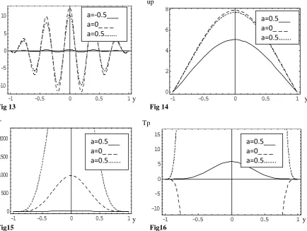
Figures (13) and (14) represent the velocities u and up for Ha = 0.5, and s = 0.5 respectively. It is clear that increasing a

increase u and up for all values of y due to the increase in velocity. It is clear that the steady state velocity attains more

than three times wall velocity due to the effects of the applied pressure gradient. Figure (15) and (16) indicate the influence of the velocity variation parameter a on the steady state profile of the temperature T and Tp, for Ha = 0.5,

S = 0.5, q = 0.1 increasing a increases both T and Tp as a result of increasing the velocities and their gradients which

increase the viscous and Joule dissipations.

Figures (17) and (18) show that variation of the velocities u and up at the centre of the channel, y = 0 with time for

different values of q, couple stress parameter and Ha = 0, S = 1, a = 0.5, It is clear that the couple stress parameter

increase both u and up increase. The figures show that increasing q increase velocity and the steady state time

Increasing the positive values of q decrease the velocity for some time and then velocity increase with increment in q as the time develops.

Figures (19), (20) show that variation of temperature T and Tp at the centre of the channel y = 0 with time for different

values of q and Ha = 0, S = 1, a = 0.5. It is clear that increasing couple stress parameter increases both T and Tp and

their steady state times.

u up

t t

Fig.1 Fig.2

T Tp

t t

Fig.3 Fig.4

Fig. 1,2,3,4 The evolation of u, up, T, Tp for different values a (H=0, s=0.q=0.1)

0 1 2 3 4

0 0.5 1 1.5 2

0 1 2 3 4

0 0.25

0.5 0.75 1 1.25

1.5 1.75

0 1 2 3 4

-300 -200 -100 0 100

0 1 2 3 4

-10 -5 0 5 10

a=-0.5____,

a=0,…………

a=0.5.---

a=-0.5____,

a=0,…………

a=0.5.---

a=0.5____,

a=0,…………

u up

Fig.5 Fig.6

T Tp

t t

Fig. 7, Fig 5,6,7,8 The evolation of u, up, T, Tp for different values a (H=1,s=0.q=0.1)

u up

t t

Fig. 9 Fig. 10

T Tp

t t

Fig.11 Fig.12

Fig 9,10,11,12 The evolution of u ,up, T, Tp for different values a (H=0,s=1.q=0.1)

0 1 2 3 4

0 2 4 6 8

0 1 2 3 4

0 2 4 6 8

0 1 2 3 4

-1.2107 -1107 -8106 -6106 -4106 -2106 0

0 1 2 3 4

-400000 -300000 -200000 -100000 0

0 1 2 3 4

0 100 200 300 400 500 600 700

0 1 2 3 4

0 0.5

1 1.5

2

0 1 2 3 4

0 2000 4000 6000 8000 10000 12000

0 1 2 3 4

-6000 -4000 -2000 0 2000 4000

a=-0.5____,

a=0,…………

a=0.5.---

a=-0.5____

a=0,…………

a=0.5.---

a=-0.5___,

a=0,…a=.5_

a=-0.5___,

a=0,…a=.5_ _

a=-0.5___,

a=0,…a=.5_ _

_{a=-0.5___,}

a=0,…a=.5_ _

a=-0.5___,

a=0,…a=.5_ _

u up

y y

Fig 13 Fig 14

T Tp

y y

Fig15 Fig16

Fig 13, 14, 15, 16, The evolution of u, up ,T, Tp for different values a (H=0.5,s=0.5.q=0.1)

u up

t t

Fig.17 Fig.18

T Tp

t t

Fig.19 Fig.20

Fig17, 18, 19 20 The evolution of u, up, T, Tp for different values q (H=0.5, s=0.5 a=0.5)

-1 -0.5 0 0.5 1

-10 -5 0 5 10

-1 -0.5 0 0.5 1

0 2 4 6 8

-1 -0.5 0 0.5 1

0 500 1000 1500 2000

-1 -0.5 0 0.5 1

-10 -5 0 5 10 15

0 1 2 3 4

0 100 200 300 400 500 600

0 1 2 3 4

0 50 100 150 200 250 300 350

0 1 2 3 4

-1.2107 -1107 -8106 -6106 -4106 -2106 0

0 1 2 3 4

-10000 -5000 0 5000 10000

a=-0.5___

a=0_ _ _

a=0.5…….

a=0.5___

a=0_ _ _

a=0.5…….

a=0.5___

a=0_ _ _

a=0.5…….

a=0.5___

a=0_ _ _

a=0.5…….

q=0.5___

q=0_ _ _

q=0.5…….

q=0.5___

q=0_ _ _

q=0.5…….

q=0.5___

q=0_ _ _

q=0.5…….

q=0.5___

CONCLUSION

In this paper the effect of a temperature dependent viscosity, suction and injection velocity, couple stress parameter, and external uniform magnetic field, on the unsteady flow and temperature distributions of an electrically conducting viscous incompressible dusty couple stress fluid between two parallel porous plates has been studied. The viscosity was assumed to vary exponentially with temperature and Joule and viscous dissipations were taken into consideration. The most interesting result was the cross-over the temperature curve due to the variation of the parameter a and influence of the magnetic field, couple stress parameter in the suppression of such cross-over on the other hand, changing the magnetic field results in the appearance of cross-over in the temperature curves for a given negative value of a. Also changing the viscosity variation parameter a leads to asymmetric velocity profiles about the central plane of the channel (y = 0) which is similar to the effect of variable percolation perpendicular to the plates.

REFERENCE

1. Stokes, V.K., the physics of fluid 3(9) PP 1709-1775. (1966).

2. Singh and Pathak., Ind. J. of pure and Appl. Math 8(6) PP. 695-701. 1977. 3. Rathod V.P., and Parveen S.R., Math Edn 3. PP 121-133, (1997).

4. Gudiraju, M., Peddieson. J., and Munukutle. S., Mechanic Research Communication 19, PP 7-13. (1992). 5. Dube. S.N., and Sharma, C.L., Phy. Soc. Japan 38. PP. 298-310 (1975).

6. Ritter J.M., and peddieson, J., Proceeding of the 6th Canadian Congress of Applied Mechanics (1977). 7. Rathod, V.P., Patel G.S., and Haq K.A., Sci. and Tech. Res GUG (1990).

8. Rathod, V.P., and Syeda Rasheeda Parveen., Int. J. Mathematical Science and Engineering Application Vol. 8 No.11, 149-160, (2014).

9. Rathod V.P., and Syeda Rasheeda Parveen., IJMA Vol. 6. No. 3, PP 11-18. (2015). 10. R.K. Gupta and S.E. Gupta., J. of Applied Mathematics and physics 27, 119. (1976). 11. P.G. Suffman., J. of Fluid Mechanics 13 PP. 120-128, (1962).

12. D.J. Tritton., physical fluid Dynamics. BLBS & Van No strand Roinhold London (1979). 13. H. Herwing .,and G. Wieken Warma., and stoffubertragung 20 PP. 47-57. (1986). 14. H.A. Attia., and N.A. Kotb., Acta Machanica 117. PP. 215-2201 No = 1, (1996).

15. G.W. Sutton.,and A. Sherman., Engineering Magnetohydrodyanamics, Mc Graw-Hill, New York, (1965). 16. W.E. Ame, Numerical Solution of partial differential Equation. 2nd ed., Academic press, New York (1977). 17. K. Klemp., H. Herwig., and M Selmann, proceedings of 3rd international Congress of fluid Mechanics, Vol. 3,

cairo, PP. 1257-1266 (1990).

Source of support: Nil, Conflict of interest: None Declared

[Copy right © 2015. This is an Open Access article distributed under the terms of the International Journal of Mathematical Archive (IJMA), which permits unrestricted use, distribution, and reproduction in any medium, provided the original work is properly cited.]