ISSN: 2347-7474
International Journal Advances in Social Science and Humanities Available online at: www.ijassh.com
RESEARCH ARTICLE
Achoka JSK et. al.| May 2016 | Vol.4 | Issue 05 |40-52
40
An Analysis of the Effect of Household Assets and Amenities
Ownership on Enrolment in Public Secondary Schools in Kenya
Wakwabubi
S, Achoka
JSK*, Shiundu
JO, Ejakait E
Masinde Muliro University of Science Technology Kenya.
Abstract
The purpose of this study was to find out whether household assets and amenities ownership has any effect on enrolment into public secondary schools in Kenya. The research design used was co-relational. The accessible study population comprised of 16,120 students from public secondary schools. A sample of 1,450 students was drawn from the population using Probability Proportion to Size (PPS) sampling technique. Questionnaires were used to collect data from the respondents. Multinomial logistic regression was used to measure the effect of household assets and amenities ownership on enrolment into public secondary schools. This study found that the number of rooms in the main house, wall, roof and floor material of this main house may affect enrolment in public secondary schools. Fetching water from rivers and springs as the main source of water for domestic use reduces the probability of joining county or national schools. Car ownership and availability of internet in the household increases the probability of joining county or national schools other than Sub county schools while DSTV connection and urban residence reduce the relative risk of enrolling in county or national schools compared with enrolling in Sub county schools. However, when other variables were controlled, this effect became insignificant and the main determinants of admission into the three categories of public secondary schools in Kenya emerged as student based-variables such as the student’s age at Kenya Certificate of Primary Education (KCPE), gender and KCPE scores .It was thus concluded that household assets and amenities ownership may not determine admission to sub-county, county or national secondary schools. Learners from the low SES category should be encouraged to work harder towards improving their academic scores in KCPE. Also they should avoid repeating classes as this does not increases the probability of such candidates being admitted to county or national secondary schools. It is recommended that that primary schools should endeavor to improve the KCPE scores of their candidates and avoid class repetition.
Keywords:
Households, Assets, Amenities, Enrollment determinants, Secondary school.
Background to the Study
Isaac [1], defined a household as a person or a group of persons, related or unrelated, who live together in the same dwelling unit, who make common provisions for food and regularly take their food from the same pot or share the same grain store, or who pool their income for the purpose of purchasing food. A household owns some assets and amenities which indicate their SES. Recent studies have shown that household SES may have effect on children education. Manheere [2] noted that children from a well-educated family with high socio-economic status are more likely to perform better than children from illiterate family. This is because the
economic status, while Patrick [4] agreed that families from different socio-economic groups create different learning environments that affect the child’s academic achievement. The research conducted by Felicia [5] based on data collected from 600 rural households provided an empirical evidence on the extent to which poverty and household demographic characteristics may affect educational attainment and school attendance of children. The results confirmed significant gender disparity in educational attainment and school attendance, with female children at a serious disadvantage.
Students whose parents have higher socio-economic status and higher levels of education may have an enhanced regard for learning, more positive ability beliefs, a stronger work orientation, and they may use more effective learning strategies than children of parents with lower socio-economic status and lower levels of education [6]. Sclafani [7] says, “A parent should begin reading to a child as soon as possible. Books provide interesting visual stimuli to infants, which forms the basis for future interest in books and reading. Keeping a child in age-appropriate books is one of the best investments any parent or grandparent can make.” Today, there is more and more emphasis on the use of television, video games, and computer games in the education of children and less and less emphasis on the simple act of reading. Parents need to go back to the basics of “providing a warm, supportive home environment that supports exploration and self-directed, autonomous behavior, and that will greatly increase the chances of having an academically successful child.” An emphasis on the parental involvement in education is the key to their children’s successful education because they are their first teachers, and therefore establish the beginning of the learning process.
Findings by the Kenya Institute for Public Policy and Research and Analysis (KIPPRA) suggested that decisions on secondary schooling are determined by social and economic characteristics such as income of parents. Also a study by United Nations, in
Tanzania, revealed that when water source was moved within 15 minutes of girl’s home, their school attendance increased by 12%.
Secondary school education is widely seen as one of the most promising avenue for individuals to realize better, more productive lives and as one of the primary drivers of national economic development. Citizens and the government of Kenya have invested heavily in improving the access, equity and quality of secondary school education, in an effort to realize the promise of education as well as to achieve the education-related Sustainable Development Goals and Vision 2030. Key goal of education is to make sure that every student has a chance to excel, both in school and in life [8]. Increasingly, children's success in secondary school education determines their success as adults, determining whether and where they go to college, what professions they enter and how much they are paid. However there are many factors preventing education from serving this role as "the great equalizer."
The Kenyan education system consists of various cycles of education. These are early childhood education, primary, secondary and tertiary. At the end of primary education, pupils sit for the Kenya Certificate of Primary Education (KCPE) examination, which determines those who proceed to secondary school or vocational training. The Ministry of Education [9] reported that form one intake entails the admission into either national, county or sub-county day schools depending on the candidate’s school choices captured during the year the candidate sat for KCPE. National schools distribute chances, based on candidature and affirmative action thus enabling each sub-county to get a candidate selected to a national school.
secondary schools intake, the public primary schools In Nairobi sent only 16 pupils (11.5%) to national schools while private schools sent 123 (88.5%) students to national secondary schools. This difference suggested that there is inequality in access to secondary school education by the type of primary school attended. Yet the common view is that increases one’s income and also plays an important role in enhancing individual’s social mobility [11]. This understanding implies that there is a need for intervention measures particularly for the poor because socio-economic background of students may have effect on the category of secondary school they attend. Knowledge on household assets and amenities, which are indicators of socio-economic status of students, in different categories of secondary schools in Kenya is a critical contribution to literature, debate and scholarship in clarifying the linkages between students’ SES and enrolment in public secondary schools in Kenya. Based on the fore going discussions of statistical data and empirical researches in the reviewed literatures, it could be evidently agreed that the household assets and amenities ownership may greatly affect the participation of children in schooling.
Statement of the Problem
In Kenya national secondary schools are top ranked followed by county and sub-county schools in descending order. Secondary schools are ranked in national examinations based on KCSE performance index. Since national schools are relatively better staffed and have adequate teaching and learning resources, they post better results in KCSE examinations compared with majority of county and sub-county schools. Due to this comparative edge in KCSE examination performance, there is bruising competition for admission into these national schools. This competition has elicited an intense public debate over which student joins national, county or sub-county secondary schools. A section of the public argues that national schools are a preserve of students from the high SES. Whereas the numbers and percentages of admission from public and private primary schools to all categories of secondary schools are known, little is
known about the effect household assets and amenities ownership on this admission in the Kenyan context. This study therefore sought to clarify the linkages between household assets and amenities ownership and enrolment to public secondary schools in Kenya.
Purpose of Study
This study set out to examine the effect of household assets and amenities ownership on enrolment in public secondary schools in Kenya.
Theoretical and Conceptual
Frameworks
This study was guided by the Social Justice Theory of John Rawls (1971). The term ‘social justice’ refers to an approach to the distribution of goods and services in society. It implies ideas of mutual obligation and a certain legal and institutional monitoring of the distribution of opportunities between citizens, such that all are given a fair and equal chance to succeed in life. The theory in particular focuses on the concept of equity and specifically on the idea of justice and fairness in the distribution of goods and services such as education.
The social justice theory advanced by John Rawls points out that due to lack of equity in the distribution of essential needs, the society has to make a choice about whether to stay with the existing laws and policies or to make changes so that equity is achieved. Authors who advocates for this theory suggests that for justice to prevail, the society should change its policies and laws to raise the position of the less advantaged members of the society.
assets and amenities they own. This study used a conceptual framework to show the relationship between independent,
dependent and control variables. The schema in figure1 shows how independent, dependent and control variables are related in this study.
Figure1: Conceptual framework showing the relationships between variables
Source: Literature Reviewed (2012/13/14)
It shows that students’ household assets and amenities ownership can potentially affect the category of secondary school they are enrolled in. Moreover, enrollment in different categories of secondary schools may be influenced by other factors such as the student’s KCPE score, sex and age, type of primary school the student attended and sat KCPE from, grade repetition and place of residence during holidays among others.
Study Design, Location of the Study
and Population
The research design used in this study was co-relational. Co-relational design helped in the assessment of the degree of relationship
that existed between the students’ household assets and amenities ownership and enrolment in different categories public secondary schools.
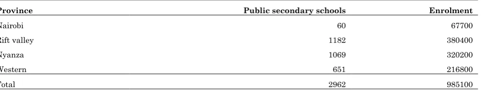
The study was carried out in Nairobi and the Western region of Kenya with the later covering the Rift valley, Nyanza and Western sub-regions. The study locations were purposively sampled because they had sufficient numbers and different categories of national schools for drawing a representative sample. The study targeted a population of 2962 public secondary schools with an enrolment of 985,100 students. Table 1 summarizes the study population disaggregated by region.
Table 1: The target population
Province Public secondary schools Enrolment
Nairobi 60 67700
Rift valley 1182 380400
Nyanza 1069 320200
Western 651 216800
Total 2962 985100
Source: Adapted from Ministry of Education(2012).PublicSecondaryschoolsp.34.[12]
The accessible study population comprised of
8,375 boys and 7,745 girls distributed in different categories of secondary schools as presented in Table 2.
Independent Variable
Household assets and amenities ownership
Dependent Variable
Category of secondary school in which a student is enrolled, which is a three level categorical variable (Sub-county, County
and National) Sub- county
County
National, which is a three level categorical variable (Low, Middle and High SES?)
Control variables
Student’s KCPE score, sex, age, type of primary school, place of residence during
Table 2: The accessible study population
Category of secondary school No of boys No. of Girls Total
National 3165 2835 6000
County 3190 2850 6040
Sub-county 2020 2060 4080
Total 8,375 7,745 16,120
Note :Adapted from Ministry of Education (2012).Public Secondary schools p.37 . [12]
Sampling Techniques and Sample
Size
Table 3 presents the number of sampled schools from the regions. A total of 18 public secondary schools were stratified and randomly sampled for this study.
Schools from each region were stratified by sex and category before being randomly sampled. The sample had six national schools, six county schools and six sub-county schools.
Table 3: Sample schools by province
Province National County Sub-county Total
Nairobi 2 1 1 4
Rift valley 3 2 2 7
Nyanza 1 2 2 5
Western 1 1 2
Total 6 6 6 18
Source: Field Work notes (2013)
Sample size was determined using a simplified formula for proportions [13] as follows:
n=𝟏+𝑵(𝒆)𝑵 𝟐
Where n = sample size, N is the population size and e is the level of precision. For national, county and sub-county schools, the sample sizes were 375, 376 and 365 as calculate below.
National schools
n=1+6000(0.05)6000 2=375 students. County schools
n=1+6040(0.05)6040 2= 376 students.
Sub-county schools
N= 4080
1+4080(0.05)2= 365 students.
Israel [14] recommends that a sample often needs to be adjusted upwards by up to 30% to cater for none response. Adjusting the sample by this percentage gave 487, 488 and 475 for national, county and sub-county schools as shown in the calculation below.
National schools
375 × 1.3 = 487 students,
County schools
376 × 1.3 = 488 students,
Sub-county schools 365 × 1.3 = 475 students.
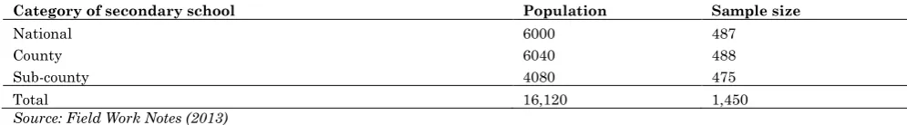
A total of 82 students were randomly sampled from each class in a school with 21 being randomly sampled from Form 1, 21 from Form 2, 20 from Form 3 and 20 from Form 4. Table 4 presents a summary of the population and the sample size.
Table 4: Accessible population and corresponding sample sizes
Category of secondary school Population Sample size
National 6000 487
County 6040 488
Sub-county 4080 475
Total 16,120 1,450
Research Instruments, Validity and
Reliability
Structured questionnaires consisting of closed ended questions were used to collect data from students. The students’ questionnaire sought information on their households’ assets and amenities ownership and category of school in which the student had been enrolled. The questionnaires consisted of five sections which were instructions for completing the questionnaire, information regarding students, information regarding parents, information regarding housing condition and amenities and information regarding household assets. A total of 1450 copies of questionnaires were used for this study.
Validity tells us whether the question, item or score measures what it is supposed to measure. To enhance validity of the research instruments, departmental research scholars ascertained that the instruments developed were valid measurements of students’ household assets and amenities ownership. Moreover, it was also important to check each item for readability, clarity and comprehensiveness.
A pilot study was done using 116 (8%) of potential respondents .A test-retest method at an interval of two weeks executed. These respondents were excluded from the actual research sample. A correlation between the initial responses and the second was made. A Pearson Product Moment Correlation formula was employed to compute the correlation coefficient in order to establish the extent to which the instruments were consistent in producing the same results. The coefficient reliability of 0.80 was achieved .This measurement was considered a high enough index of reliability. Accordingly, the instrument was used for data collection.
Data Analysis
Data were analyzed using both descriptive and inferential statistics. Descriptive statistics were used to determine means, median, standard deviation, variance, skewness, kurtosis, range and frequencies. A sequential multinomial logistic regression
was fitted to model the effect of student household assets and amenities ownership on enrolment to different categories of secondary schools. Multinomial Logistic Regression (MLR) was preferred because the dependent variable was a three level categorical variable and it allowed simultaneous comparison of more than one alternative.
That is, the Relative Risk Ratio (RRR) of the alternatives were estimated simultaneously by comparing enrolment to national and county schools with that in sub-county schools which was the reference category, also called the base category. For each model, MLR ran regressions for the relative risk of enrolment to county secondary school versus sub-county secondary school and national secondary school versus sub-county secondary school. Multinomial logistic regression also gives separate coefficient estimates for each independent variable for each category of comparison. The estimated coefficients represented the relative risk of being in the comparison category versus being in base category associated with a one unit increase in the independent variable. The multinomial logistic model took the form:
𝑃𝑟(𝑦
𝑖= 𝑗) =
𝑒𝑥𝑝(𝑋
𝑖𝛽
𝑗)
1 + ∑
𝑗𝑗=1𝑒𝑥𝑝(𝑋
𝑖𝛽
𝑗)
Where i is the respondent, yi is the observed outcome, Xi the independent variables and βj are the beta coefficients that are estimated using maximum likelihood. Once the coefficients are exponentiated they give odds ratios (OR) reported as the RRR in MLR. The beta coefficients βj are interpreted as the increase in Relative Risk Ratio of being in category j versus the base category resulting from a one-unit increase in the ith covariate, holding the other covariates constant. In this case, βj are the increases in relative risk of admission or enrolment in county or national secondary schools versus admission or enrolment in sub-county schools.
Findings and Discussions
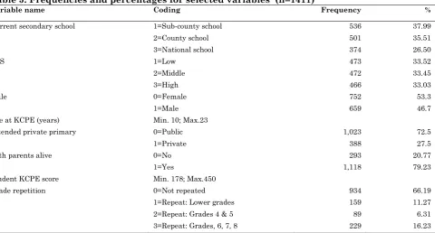
enrolment into different categories of public secondary schools, the preferred statistical approach was to fit MLR models because the dependent variable was an un-ordered three-level categorical variable. But first, frequencies, percentages and descriptive statistics of the variables used in the analysis are given. Table 5 presents frequencies and percentages of selected variables used in the regression analysis. The results show that 37.99% of the students were from sub-county secondary schools, 35.51% of the students were from county secondary schools and 26.50% of students were from national secondary schools. The table also shows that there were 473 (26.50%) from low SES, 472 (33.45%) from middle SES and 466 (33.06%) from high SES. This suggested that
there was a fair distribution of students in sample from low, middle and high SES. As expected, the results also show that the number of orphans and students with single parent were fewer (20.77%) compared to students who had both parents alive (79.23%). The findings further revealed that grades 6, 7 and 8
were most affected by grade repetition with 229 sampled students responding that they repeated those grades compared with 89 who repeated at grade 4 or 5. This is expected because repetition in higher classes is probably meant to improve the final KCPE score. Moreover we found that that a higher proportion of students enrolled in public secondary school were from public primary schools at 72.5% compared to 27.5% of students from private primary schools.
Table 5: Frequencies and percentages for selected variables (n=1411)
Variable name Coding Frequency %
Current secondary school 1=Sub-county school 536 37.99
2=County school 501 35.51
3=National school 374 26.50
SES 1=Low 473 33.52
2=Middle 472 33.45
3=High 466 33.03
Male 0=Female 752 53.3
1=Male 659 46.7
Age at KCPE (years) Min. 10; Max.23
Attended private primary 0=Public 1,023 72.5
1=Private 388 27.5
Both parents alive 0=No 293 20.77
1=Yes 1,118 79.23
Student KCPE score Min. 178; Max.450
Grade repetition 0=Not repeated 934 66.19
1=Repeat: Lower grades 159 11.27
2=Repeat: Grades 4 & 5 89 6.31
3=Repeat: Grades, 6, 7, 8 229 16.23
Source: Analysis of Data (2013)
The findings also revealed that the range of age at KCPE is a bit wide from 10 years old to 23 years old. This range could probably be attributed to introduction of free primary education and free day secondary education by the government of Kenya in 2003 and 2008 respectively which prompted re-enrolment in secondary schools by some students who had probably dropped out of schools for various reasons. Table 6 presents selected descriptive
statistics for selected variables. Measures of central tendency (mean and median) for selected variables were computed to summarize and give a figure which represents the whole data. Age at KCPE had a mean of 14.51, median of 14, Std. Dev. of 1.13, variance of 1.87 and range of 10 to 23.
deviation, variance and range suggested that there was some variation in the age at KCPE. Age at KCPE was one of student based control variable used in this study for examining the effect of student SES on enrolment in public
secondary schools. Out of the possible 500 KCPE score, the sample had scores ranging from 178 to 450 scores. There was some variability in the KCPE scores as suggested by a standard deviation of 56.58.
Table 6: Selected descriptive statistics for selected variables
Variable Mean Median Std. Dev. Variance Skewness Kurtosis Obs. Range Min Max
Age at KCPE 14.51 14 1.37 1.87 0.88 5.10 1442 13 10 23
Student KCPE score 335.09 337 56.58 3201.16 -0.12 2.07 1448 272 178 450
Note: Std. Dev. = Standard deviation, Obs. =Observations, Min. =Minimum, Max. =Maximum. Source: Analysis of Data (2013)
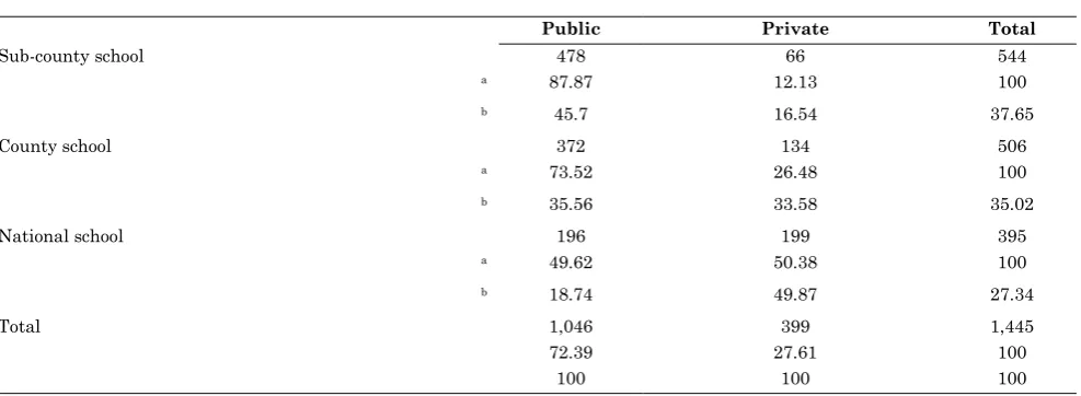
Table 7 Presents Chi square test between students’ secondary school of
enrolment and type of primary school attended.
Table 7: Chi square test between current secondary school of enrolment and students’
primary school of origin (n=1445)
Current secondary school Type of primary school attended
Public Private Total
Sub-county school 478 66 544
a 87.87 12.13 100
b 45.7 16.54 37.65
County school 372 134 506
a 73.52 26.48 100
b 35.56 33.58 35.02
National school 196 199 395
a 49.62 50.38 100
b 18.74 49.87 27.34
Total 1,046 399 1,445
72.39 27.61 100
100 100 100
Note. a=row percentages; b=column percentages Pearson chi2(2) = 167.9785, p< .001; Cramer's V 0.34 Source: Analysis of Data (2013)
The findings reveal that a bigger proportion (87.87% for sub-county secondary schools and 73.52% for county secondary schools) of students joining sub-county and county secondary schools is from public primary schools. However, the distribution of students from public and private primary schools in the national schools is approximately the same (49.62% from public primary schools and 50.38% from private primary schools).This findings discount findings by the International Finance Corporation (IFC) in the year 2002 about “The business of Education: A look at Kenya’s private education sector which found out that in the 2001 secondary
schools intake , the public primary schools In Nairobi sent only 16 pupils (11.5%) to national schools while private schools sent 123 (88.5%) students to national secondary schools.
significance value, the researcher was able determine whether the correlations were significant. The null hypothesis was that the correlation coefficient is zero and could be rejected at a 5% significance level. Most of the variables are significantly correlated at p<.001. The dependent variable (Current secondary school of enrolment) has a moderate positive correlation of 0.43 with the independent variable (SES). The 0.85 positive correlation between the current secondary school of enrolment and the student’s KCPE score is the strongest. Other positively correlated variables are type of
primary school and current secondary school at 0.34, SES and current secondary school at 0.43, type of primary school and SES at 0.38, student KCPE score and SES at 0.43 and student KCPE score and type of primary school at 0.35. The highest negative correlation was between age at KCPE and current secondary school at - 0.53.These correlations showed the existence of relationship between the variables. Because of these relationships, the variables were fitted into a sequential MLR model to measure the magnitude of effect each of these variables on the dependent variable.
Table 8: Pair-wise correlations between variables showing significance at 5% level of significance
S.No. Variable name 1 2 3 4 5 6 7 8
1 Current secondary school 1
2 SES 0.43*** 1
3 Both parents alive 0.14*** 0.16*** 1
4 Type of primary 0.34*** 0.38*** 0.09* 1
5 Male -0.06* -0.02* -0.00 -0.02 1
6 Age at KCPE -0.53*** -0.31*** -0.12*** -0.24*** 0.18*** 1
7 Grade repetition -0.36*** -0.18*** -0.04 -0.16*** -0.03 0.42*** 1
8 Student KCPE score 0.85*** 0.43*** 0.12*** 0.35*** 0.09** -0.49*** -0.41*** 1
*p<.05, **p<.01,***p<.001 Source: Analysis of Data (2013)
Multinomial Logistic Regression
Coefficients of Household Amenities
and Assets Ownership Factors on
Admission to Sub-county, County or
National Secondary Schools
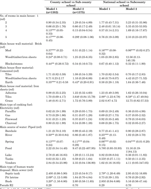
Table 9 presents the MLR coefficients of the individual household SES variables on enrolment in Sub county, county or national public secondary school. Just like in question two, a sequential multinomial logistic regression model was fitted to estimate the effect of variables on individual ownership of household assets and amenities available to the households on enrolment in Sub county, county or national school while controlling for parent and pupil level variables. Model 1 fits the dependent variable (current secondary school of enrolment) and independent SES variables on individual ownership of household assets and amenities. As controls, model 2 introduces student-based variables such as the type of primary school where the student sat KCPE from, the age of the student at KCPE, grade
has an earthen floor, the relative risk of joining a county school other than a Sub county school would reduce by a RRR of
0.35, p<.001 in model 1 and 0.43, p<.001 in model 2 after introducing the control variables.
Table 9: Multinomial logistic regression coefficients of household amenities and assets ownership factors on admission to sub-county, county or national secondary schools (n=1222, 95% confidence interval in parenthesis)
County school vs Sub county school
National school vs Subcounty school
Model 1
(n=1382) Model 2 (n=1375) Model 1 Model 2
No. of rooms in main house: 1 (ref)
2 0.90 (0.34-2.35) 1.29 (0.34-4.89) 1.77 (0.43-7.31) 3.23 (0.31-33.86)
3 0.66 (0.25-1.76) 0.66 (0.17-2.49) 2.48 (0.61 10.14) 5.35 (0.53-53.93)
4 0.13***
(0.05-0.33) 0.15 (0.04-0.54) 0.57 (0.14-2.31) 1.69 (0.16-17.67)
5 0.17***
(0.06-0.45) 0.29† (0.08-1.06) 0.76 (0.19-3.09) 2.33 (0.23-23.97)
Main house wall material: Brick (ref)
Mud 0.37***
(0.22-0.64) 0.51 (0.22-1.14) 0.16*** (0.08-0.32) 0.06*** (0.02-0.27)
Wood/timber/iron sheets 0.24* (0.08-0.71) 1.25 (0.25-6.35) 1.05 (0.39-2.85) 12.56
(0.13-140.19)
Blocks/stones 0.44** (0.26-0.72) 0.34 (0.16-0.73) 0.67 (0.40-1.12) 0.32 (0.11-1.90)
Main house floor material: Cemented (ref)
Tiles 1.71 (0.82-3.59) 1.08 (0.34-3.39) 1.70 (0.82-3.54) 0.70 (0.17-2.83)
Wood/timber/iron sheets 0.71 0.23-2.17 1.16 (0.20-6.88) 2.46 (0.75-8.07) 4.42 (0.27-71.52)
Earth 0.35*** 0.21-0.58 0.43* (0.20-0.91) 0.58 (0.28-1.18) 1.64 (0.36-7.46)
Main house roof material: Iron sheets (ref)
Asbestos 0.88 (0.35-2.25) 1.22 (0.32-4.60) 1.23 (0.49-3.08) 1.62 (0.26-10.04)
Tiles 1.70 (0.69-4.17) 3.64† (0.84-15.79) 2.88* (1.23-6.78) 8.58* (1.47-49.94)
Grass 1.48 (0.81-2.71) 1.72 (0.76-3.89) 2.02 0.87-4.72 12.75 (0.82-57.53)
Main type of cooking fuel: Electricity (ref)
Paraffin 0.62 (0.19-1.99) 0.29 (0.05-1.73) 0.69 (0.19-2.49) 0.36 (0.03-4.98)
Gas 0.73 (0.29-1.86) 0.31 (0.07-1.28) 0.69 (0.27-1.75) 0.37 (0.05-2.52)
Firewood 0.51 (0.21-1.28) 0.3† (0.07-1.24) 0.92 (0.35-2.46) 0.79 (0.10-6.03)
Charcoal 0.80 (0.32-1.98) 0.34 (0.09-1.38) 0.68 (0.26-1.75) 0.32 (0.05-2.27)
Main source of water: Piped (ref)
Borehole 1.21 (0.70-2.10) 0.99 (0.45-2.19) 0.77 (0.41-1.41) 0.90 (0.28-2.87)
River 0.50** (0.30-0.84) 0.86 (0.40-1.87) 0.25***
(0.13-0.48) 1.02 (0.28-3.70)
Spring 0.13***
(0.07-0.24)
0.11*** (0.04-0.29)
0.06*** (0.02-0.15)
0.04*** (0.01-0.20)
Pond 2.22 (0.34-14.40) 9.47 (0.22-407.95) 5.78† (0.93-35.93) 15.16
(0.19-1184.13)
Lake 2.78 (0.46-16.83) 1.29 (0.11-15.24) 0.82 (0.08-8.04) 0.36 (0.01-11.82)
Tanks 0.63 (0.32-1.25) 0.59 (0.21-1.64) 0.55† (0.27-1.11) 0.50 (0.11-2.35)
Vendors 2.84 (0.34-23.96) 2.35 (0.04-136.90) 1.62 (0.16-16.05) 4.11 (0.05-347.05)
Main type of human waste disposal: Main sewer (ref)
Septic tank 2.40† (0.98-5.90) 2.23 (0.54-9.17) 2.79* (1.20-6.49) 2.95 (0.52-16.69)
Pit latrine 2.09* (1.12-3.89) 1.84 (0.70-4.84) 0.73 (0.39-1.35) 0.76 (0.20-2.92)
Bush 3.20* (1.16-8.80) 2.60 (0.58-11.65) 2.85† (0.94-8.66) 5.16 (0.56-47.44)
Pseudo R2 0.29 0.70 0.29 0.70
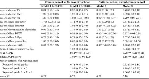
Table 9: Continued
County school vs Subcounty school National school vs Subcounty school
Model 1 (n=1382) Model 2 (n=1375) Model 1 Model 2
Household owns TV 0.84 (0.50-1.41) 0.96 (0.45-2.07) 0.64 (0.33-1.28) 0.78 (0.19-3.16)
Household owns DVD 1.25 (0.75-2.07) 1.26 (0.59-2.71) 0.90 (0.49-1.69) 0.62 (0.18-2.13)
Household owns car 1.39 (0.86-2.23) 1.93† (0.93-4.00) 2.02** (1.21-3.37) 2.79† (0.98-7.94)
Household has computer 1.76† (0.98-3.17) 1.12 (0.46-2.74) 1.33 (0.70-2.50) 0.87 (0.25-2.96)
Household has internet 1.23 (0.71-2.11) 1.05 (0.45-2.49) 2.25** (1.26-4.02) 1.34 (0.43-4.16)
Household connected to electricity 0.97 (0.60-1.57) 1.39 (0.66-2.93) 1.37 (0.77-2.45) 1.53 (0.46-5.11)
Household has DSTV 0.62 (0.34-1.12) 0.52 (0.21-1.30) 0.40** (0.21-0.76) 0.27* (0.08-0.94)
Household has fridge 0.73 (0.42-1.26) 0.78 (0.35-1.77) 0.98 (0.54-1.78) 2.57 (0.75-8.80)
Household has gas cooker 1.30 (0.82-2.06) 0.68 (0.34-1.38) 1.31 (0.77-2.22) 0.35† (0.12-1.06)
Household owns cattle 0.87 (0.60-1.27) 1.47 (0.82-2.63) 0.49** (0.33-0.75) 1.20 (0.52-2.78)
Attended private primary school 1.22 (0.66-2.25) 0.96 (0.40-2.31)
Age at KCPE 0.52*** (0.43-0.64) 0.28*** (0.19-0.41)
Student KCPE score 1.06*** (1.05-1.09) 1.18*** (1.16-1.20)
Grade repetition: Not repeated (ref)
Repeated lower grades 0.72 (0.37-1.38) 0.92 (0.30-2.84)
Repeated grade 4 or 5 1.89 (0.75-4.75) 1.29 (0.23-7.33)
Repeated grade 6 or 7 or 8 1.10 (0.58-2.08) 1.36 (0.29-6.40)
Pseudo R2 0.29 0.70 0.29 0.70
Note: †p<.10, *p<.05, **p<.01,***p<.001 Source: Analysis of Data (2013)
Since it is cheaper to build houses with mudded walls and earthen floors, households owning these kind of houses as their main houses may be considered humble and therefore belonging to the low SES. Perhaps the inferential meaning from these results would be that the relative risk of joining county or national schools other than Sub county ones for students from such humble and low SES is reduced, meaning that the relative risk of such students joining a Sub county school is increased.
With the reference category as iron sheets, students whose main houses are roofed with tiles are more likely to enroll in a county or national school than a Sub county school with relative risk ratios of 3.64, p=.085 and 8.58, p=.017 respectively after introducing the control variables. This result seems to support the earlier finding on mudded walls and earthen floors and suggests that since it is perhaps more expensive to build a tile-roofed house than say, one with iron sheets, students from such homes would be considered to be in the middle or high SES categories and their relative risk of joining a county or national school would be enhanced. It is however difficult to maintain this argument because after introducing
control variables, the relative risk of joining a national school other than a Sub county one for students from grass thatched homes is also increased by a RRR of 12.75, p=.001.
With the reference source as piped water into the compound, the relative risk of joining county or national schools is reduced by 0.13, p<001 and 0.06, p<001 respectively in model 1 and by 0.11, p<001 and 0.04,
p<001 respectively in model 2 for students whose households main source of water is the spring or river. With many students in the sample residing in the rural areas, this would be expected since the students would most probably be the ones fetching water from rivers and springs than older household members. It would take much longer to do this from rivers and springs than from taped water into the compound. The inference is that considerable time is used on household chores, leaving little time for academic work while at home. This would lead to low KCPE scores and as seen earlier, low scores reduce the probability of joining county or national schools.
whose households own a car by a RRR of 1.93, p=.077 and 2.79, p=.055 respectively.
Households that have DSTV reduce the relative risk of their class 8 students joining county or national schools. Such students are more likely to join Sub county schools.
This is not a strange finding because excessive watching of DSTV programming by students at the expense of academic work is likely to lead to low or poor scores in KCPE. Such scores reduce the probability of enrolling in “good” schools. Surprisingly, urban residence reduces the relative risk of enrolling in county or national schools by 0.42, p<001 and 0.40, p=.001 in model 1 respectively and 0.36, p=.004 and 0.27,
p=.015 in model 2 respectively. In the full model (2) when control variables are introduced, a one-year increase in age reduces the relative risk of enrolling in a county or national school by 0.52, p<001 and 0.28, p<001 respectively. A one-point/mark increase in the KCPE score increases the relative risk of enrolling in a county or national school by 1.06, p<001 and 1.18,
p<001 respectively.
These effects were also observed in research question 2. Again, grade repetition is insignificant. The Pseudo R2 in model 1 is 0.29. In model 2, there is a massive improvement to 0.70 denoting that the introduction of student level control variables massively strengthened the final model. This is in agreement with the findings in question 1 which showed that when control variables were introduced, the effect of SES became insignificant. The Pseudo R2 is the proportion of variance for the response variable explained by the predictors and ranges between 0 and 1 with 1 denoting 100% explanation of the response variable.
These findings may point in the same direction as those found by the Kenya Institute for Public Policy and Research and Analysis (KIPPRA) (2006) that suggested that decisions on secondary schooling are determined by social and economic characteristics such as income of parents. These findings are also in tandem with study by United Nation (1995) that in Tanzania, when water source were moved within 15 minutes of girls home, their school attendance increased by 12% [15-16].
Conclusions
The purpose of this study was to find out whether household assets and amenities ownership of the students has any effect on enrolment into public secondary schools in Kenya. The study concludes that household assets and amenities ownership does not determine enrolment into public secondary. Instead, it is student-based variables such as the sex of the student, age at KCPE and the student’s KCPE score that are the determinants of enrolment in public secondary schools in Kenya.
Recommendations
The following are the recommendations derived from the study findings:
That primary school should seek to
improve the KCPE scores of their candidates as this increases the probability of such candidates being admitted to county or national schools.
That since household assets and amenities
ownership does not determine admission to sub-county, county or national schools, students from the low SES category should be encouraged not to look down upon their household assets and amenities ownership and instead be encouraged to work at improving their scores in KCPE.
References
1 Isaac D, Ephraim NP (2004) Characteristic of Households and Household members. Retrieved from http//www.dhsprogram.com. 2 Menheere, A, Edith HH (2012) Parental
involvement in children‟s education: review study about effect of Parental involvement on children’s School education with a focus on the
position of illiterate parents. Journal of the European Teacher Education Network Jeten, 6:148.
4 Patrick AO (2012) School Dropout among senior Secondary schools in Delta state University Abraka, Nigeria.
5 Felicia IO (2001) Female access to basic education: A case for open Distance Learning (ODL).
6 Joan MT, Smrekar CW (2009) Influence of Parents' level of Education, Influence on Child's Educational Aspirations and Attainment.
7 Sclafani Joseph D (1994)The Educated Parent: Recent Trends in Raising Children Connecticut: Praeger Publishers, 2004
8 Valarie EL, David TB(2002) Inequality at the Starting Gate. Retrieved from http://www.Epi.org/content.cmf?id
9 Ministry of Education (2013) Form One Selection. Retrieved from http://www.education.go.ke
10 Epari E, Maurice M, Alex E, Moses E, Moses O, Moses N (2011) Factors associated with low achievement amoung students from nairobis urban informal neiborhoods. Urban Education, 42(5):1056-1077.
11 Psacharapoulos G, Woodhall M (1985) Education for Development. Analysis of Investment choices, Washington D.C.: Oxford University Press.
12 Ministry of Education (2012).Public Secondary schools .Retrieved from http://www.education.go.ke
13 Yamane T (1967) Statistics, An Introductory Analysis, 2nd Ed., New York: Harper and Row, p.887.
14 Israel GD (1992) Sampling The Evidence Of Extension Program Impact. Program Evaluation and Organisation Development, IFAS, University of Florida.PEOD-5October. 15 Bulimo AW (2009) Equity in Access to
Secondary by Private and Public Primary Schools Gratuate in Kakamega South Sub-county, Kenya. (Unpublished masters dissertation). Masinde Muliro University of Science and Technology, Kakamega.