brain labeling
Guangkai Ma
Space Control and Inertial Technology Research Center, Harbin Institute of Technology, Harbin 150001, China and Department of Radiology and BRIC, University of North Carolina at Chapel Hill,
Chapel Hill, North Carolina 27599
Yaozong Gao and Guorong Wu
Department of Computer Science, Department of Radiology, and BRIC, University of North Carolina at Chapel Hill, Chapel Hill, North Carolina 27599
Ligang Wu
Space Control and Inertial Technology Research Center, Harbin Institute of Technology, Harbin 150001, China
Dinggang Shena)
Department of Radiology and BRIC, University of North Carolina at Chapel Hill, Chapel Hill, North Carolina 27599 and Department of Brain and Cognitive Engineering, Korea University, Seoul 02841, Republic of Korea
(Received 1 September 2015; revised 17 December 2015; accepted for publication 10 January 2016; published 2 February 2016)
Purpose:It is important for many quantitative brain studies to label meaningful anatomical regions in MR brain images. However, due to high complexity of brain structures and ambiguous boundaries between different anatomical regions, the anatomical labeling of MR brain images is still quite a challenging task. In many existing label fusion methods, appearance information is widely used. However, since local anatomy in the human brain is often complex, the appearance information alone is limited in characterizing each image point, especially for identifying the same anatomical structure across different subjects. Recent progress in computer vision suggests that the context features can be very useful in identifying an object from a complex scene. In light of this, the authors propose a novel learning-based label fusion method by using both low-level appearance features (computed from the target image) and high-level context features (computed from warped atlases or tentative labeling maps of the target image).
Methods: In particular, the authors employ a multi-channel random forest to learn the nonlinear relationship between these hybrid features and target labels (i.e., corresponding to certain anatomical structures). Specifically, at each of the iterations, the random forest will output tentative labeling maps of the target image, from which the authors compute spatial label context features and then use in combination with original appearance features of the target image to refine the labeling. Moreover, to accommodate the high inter-subject variations, the authors further extend their learning-based label fusion to a multi-atlas scenario, i.e., they train a random forest for each atlas and then obtain the final labeling result according to the consensus of results from all atlases.
Results:The authors have comprehensively evaluated their method on both public LONI_LBPA40 and IXI datasets. To quantitatively evaluate the labeling accuracy, the authors use the dice similarity coefficient to measure the overlap degree. Their method achieves average overlaps of 82.56% on 54 regions of interest (ROIs) and 79.78% on 80 ROIs, respectively, which significantly outperform the baseline method (random forests), with the average overlaps of 72.48% on 54 ROIs and 72.09% on 80 ROIs, respectively.
Conclusions: The proposed methods have achieved the highest labeling accuracy, compared to several state-of-the-art methods in the literature. C 2016 American Association of Physicists in Medicine.[http://dx.doi.org/10.1118/1.4940399]
Key words: MR brain image labeling, multi-channel, nonlinear learning, context model, random forests
1. INTRODUCTION
Many quantitative brain image analyses often rely on the reliable labeling of brain images.1–5Thus, automatic labeling
of brain MR images becomes a notable topic in the field of medical image analysis. Due to the burden of manual brain
1004 Maet al.: Nonlocal atlas-guided multi-channel forest learning 1004
Among all the existing brain labeling techniques, multi-atlas based labeling methods have achieved great success recently. In these methods, a set of already-labeled brain MR images, namely, atlases, is used to guide the labeling of new target images.6–9Specifically, given a target image to
be labeled, multiple atlas images will be first warped onto the target image, and then the estimated warping functions will be applied to transforming their corresponding label maps to the target image. Finally, all warped atlas label maps will be fused for labeling the target image. The performance of multi-atlas based labeling methods depend on both the accuracy of registration and the effectiveness of the label fusion step. Since image registration is also a challenging problem in the medical image analysis area,10,11 more researchers are focusing on improving the labeling performance by proposing more effective label fusion techniques.12,13 For example, Coupé et al.12proposed a nonlocal patch-based label fusion technique by using patch-based similarity as weight to propagate the neighboring labels from aligned atlases to the target image, for potentially overcoming errors from registration. Instead of pair-wisely estimating the patch-based similarity for label fusion, Wu et al.13 proposed to use sparse representation to
jointly estimate all patch-based similarities between a to-be-labeled target voxel and its neighboring voxels in all atlases. However, the traditional multi-atlas based labeling techniques suffer fromtwo limitations: (1) the definition of patch-based similarity is often handcrafted based on predefined features (e.g., image intensity), which may not be effective for labeling all types of brain structures; (2) only a linear prediction model is often used for propagating labels of aligned atlases onto the target image, thus potentially limiting the labeling accuracy.
On the other hand,learning-based labeling methodshave also attracted significant attention recently. In the learning-based methods, a strong classifier, such as support vector machine (SVM),14Adaboost,15random forests,16and artificial
neural networks,17is typically trained for each label/region of
interest (ROI) in the brain image, based on the local appearance features. In the testing stage, the learned classifiers are applied to voxel-wisely classifying the target image. The label of each voxel is then determined as the class with the largest classification response on that voxel. These learning-based labeling methods can fully use the appearance information of a target image for labeling, through extraction of abundant texture information from a local image patch. In the testing stage, the learned classifiers are applied to voxel-wisely classifying the target image. The label of each voxel is then determined as the class with the largest classification response on that voxel. These learning-based labeling methods can fully use the appearance information of a target image for labeling, through extraction of abundant texture information from a local image patch. For example, Zikicet al.18proposed atlas
forest, which encodes an atlas by learning a classification forest on it. The final labeling of a target image is achieved by averaging the labeling results from all selected atlas forests. Tu and Bai19 adopted the probabilistic boosting tree (PBT)
with Haar features and texture features for labeling MR brain images. To further boost labeling performance, an
auto-context model (ACM) was also proposed to iteratively refine the labeling results. Compared to the global learning of a classifier for labeling the entire ROI, Haoet al.20 proposed a local label learning method for labeling each target voxel with the online learning classifier, which is trained with k nearest neighbor (k-NN) training samples of the target voxel from the aligned atlases. However, the online learning manner is often time-consuming, which limits the utilization of sophisticated classification algorithms, and subsequently affects the segmentation accuracy of complex brain structure. Overall, themajor concernwith the learning-based labeling methods is that the spatial information of labels encoded in the atlases is not fully utilized. Moreover, in contrast to the multi-atlas based labeling methods described above, the learning-based labeling methods often determine a target voxel’s label based solely on the local image appearance, without receiving clear assistance from the aligned atlases. Accordingly, their labeling accuracy can be limited, since patches with similar local appearance could appear in different parts of the brain. Although Zikicet al.18utilized the population mean atlas for
learning atlas forests, due to large intersubject variations, the structural details in the constructed population-mean atlas are lost, thus hindering the accurate labeling of brain structures. Besides, in comparison to other learning-based methods, atlas forest is prone to overfitting, as it learns a strong classifier from only a single brain image, not from a set of brain images as typically done in other approaches.19,20Specifically, if the
target image is anatomically different from several atlases in the library, the classification forests trained on those atlases will degrade the final labeling result of the target image.
In this paper, we propose a novel atlas-guided multi-channel forest learning method for labeling multiple ROIs. Here, multi-channel refers to multiple representations of a target image, which include features extracted from not only the target (intensity) image but also the label maps of all aligned atlases. Specifically, instead of labeling each target voxel with only its local image appearance from the target image, we also utilize label information from the aligned atlas.
• In the training stage, we first train an atlas-specific clas-sification forest for each atlas, along with the (training) target image. Note that the atlas-specific classifier is trained based on the local image appearance of this voxel in the (training) target image as well as the label informa-tion of the aligned atlas, which effectively avoids missing any spatial label information of the target voxel, as in the existing learning-based labeling methods. Different from previous multi-atlas based methods,12,13 which
iteratively construct a sequence of classification forests by updating local label context features from the newly estimated label maps for training.
• In the testing stage, each atlas-specific classification forest is independently applied to estimate class prob-ability for each voxel in the (test) target image. The final labeling result is the average of all labeling results from all atlas-specific forests. Specifically, given an aligned atlas, which includes its associated atlas-specific classification forest and a target voxel in the (test) target image, we first findk-NN voxels of the target voxel in the aligned atlas. Then, for each of the k-NN voxels, its label features are extracted from the aligned atlas, and further combined with the local image appearance of the target voxel, as input to the learned forest for classification. Finally, the labeling results from all k -NN voxels are averaged to obtain the labeling result of the target voxel using this atlas-specific forest. Once the tentative labeling result of the target image is obtained by averaging all atlas-specific forests, the label features originally computed from each aligned atlas will be now replaced by those computed from the tentative labeling result/map for iterative classification refinement with the proposed HMCCM. Validated on both LONI_LBPA40 and IXI datasets, our proposed method consistently outperforms both traditional multi-atlas based methods and learning-based methods.
Finally, we want to mention that the preliminary version of this work appeared in Ref.21. Compared with the previous work, we present two novelties in the method as described below. Moreover, we extensively evaluate the sensitivity of our method with respect to different parameters and also validate our method in an additional IXI dataset.
• In the previous work, we extracted features from the corresponding voxels in the atlases, without considering potential registration errors. In this paper, we propose a nonlocal strategy to relieve labeling mistakes brought by registration errors.
• We further present a HMCCM to replace original label features from the aligned atlases, which can produce more accurate label information through an iterative scheme.
The rest of the paper is organized as follows. Section 2 describes the proposed labeling method and its application to single-ROI and multi-ROI labeling. Experiments are performed and analyzed in Sec. 3. Finally, discussion and conclusion are given in Sec.4.
2. METHOD
In this section, we will first present notations used in our pa-per. Then, we will explain the learning procedure of our atlas-guided multi-channel forest, followed by the application of learned forests to single-ROI and multi-ROI labeling. Finally, we present HMCCM to iteratively refine the labeling results.
2.A. Notations
An atlas library A consists of multiple atlases {Ai
=(Ii,Li)|i=1,...,N}, whereIiandLiare the intensity image
and the label image/map of theith atlas, and N is the total number of atlases in the library A. SetT={Tj=(Hj,Bj)|j
=1,...,M}represents the training set, whereHjandBjare the
intensity image and the label image/map of the jth training sample, and M is the total number of training samples. Aij={Iij,Lij},i=1,...,N,j=1,...,M denotes the intensity(Iij) and label(Lij)images of theith atlas after mapping to the jth training image. Each brain ROI is assigned with a ROI/label s,s=1,...,S, whereSis the total number of ROIs.Psdenotes
the label probability map of ROIs. Here, we usexto denote the coordinate of a voxel andck(x)to denote the coordinate of
thekth nearest voxel of the voxelx.
2.B. Atlas-guided multi-channel forest learning
To increase the flexibility of our learning procedure, we will train one multi-channel random forestFi,s(i.e., multi-channel
forest) for each atlasi and each ROI s. In this way, when a new atlas is added into the atlas libraryA, only the new multi-channel forest needs to be trained with the new atlas, while all previously trained forests can be reused. To label a single ROI, N multi-channel forests (corresponding toN atlases) will be learned, with each trained forest corresponding to a specific atlas. Section2.C will show how the multi-channel forests of different ROIs can be combined effectively for multi-ROI labeling. In this section, we focus on the learning part of our method.
To label one ROI, i.e., the sth ROI, during the training stage, we will learn a multi-channel forest Fi,s for each
atlas, i.e., theith atlas. Due to anatomical variability between individual brains, there is often inconsistency between the label information provided by atlas and the actual label in the target image. To obtain more accurate label information from the atlas for labeling, registration and patch selection are performed as follows. First, during the learning of the ith atlas-specific forest, we nonrigidly register the ith atlas imageIi onto each training target image Hj, and then also
obtain the warped atlas label map Lij by applying the same estimated transformation on the atlas label map Li. In this
way, M training image pairs {Hj,Iij,Lij,Bj},j=1,...,M are
formed, whereHj,I j i, andL
j
i are used for extracting features
while the label mapBj is used to provide the class label for
forest learning. Afterward, the positive and negative samples are taken inside and outside of thesth ROI from every training image pair for multi-channel forest learning, as detailed below.
• For each sample voxel x in the training image Hj,
we first extract its appearance features from a local patch of the training image Hj, centered at x. To
reduce the registration error and further acquire more accurate label from the atlas, according to the similarity between local intensity patches of training image and warped atlas image, we search a nearest voxelc1(x)ofx
1006 Maet al.: Nonlocal atlas-guided multi-channel forest learning 1006
F. 1. The flowchart of our method for learning one multi-channel forest with theith atlas. An example for sample selection during the training stage is also given in the right-bottom corner, where blue points denote samples belonging to the ROI while green points denote samples belonging to the background. Note here that more samples are drawn around the ROI boundaries.
label image Lij. Finally, both appearance features and label features are combined to jointly characterize the appearance and spatial label context information of each sample voxel and are used for inferring label.
• After training, N multi-channel forests (corresponding to N atlases) will be learned for each ROI. Thus, in total, S×N multi-channel forests will be obtained for all S ROIs under labeling. The flowchart shown in Fig.1gives an illustration for learning one multi-channel forest.
Sampling strategy:The positive and negative samples used to train multi-channel forest for the sth ROI are randomly sampled inside and outside the sth ROI, respectively. To effectively classify voxels near the ROI boundary and also to avoid data imbalance between positive and negative samples, we select positive and negative samples near the boundary of the target ROI, as shown in the right bottom of Fig. 1. Intuitively, voxels around the ROI boundary are more difficult to be correctly classified than other voxels. Therefore, more samples should be drawn around the ROI boundary during the sampling stage. In our implementation, voxels that lie in the areas within 2 voxels from the ROI boundary account for 80% of total training samples. The numbers of positive and negative samples are kept the same.
Feature extraction:To train multi-channel forests for the ith atlas, as mentioned above, every training imageHjwill be
associated with its respective alignedith atlasAij={Iij,Lij}(on the jth training image space). Note that the features of each sampled voxel, used to train our multi-channel forest Fi,s,
come from both the training image and the alignedith atlas label map. More specifically, there areS+1 different channels of features extracted for each sampled voxel: 1 channel of local appearance features of this voxel extracted from the training image (e.g.,Hj), andS channelsoflocal label context
featuresof the corresponding voxel extracted from the aligned ith atlas label map (e.g.,Lji) with respect to each ofSROI.
Local appearance features: The local image appearance features extracted from a given (training) target image include (1) patch intensities within a 11×11×11 neighborhood, (2) outputs from the first-order difference filters (FODs), second-order difference filters (SODs), 3D Hyperplane filters, 3D Sobel filters, Laplacian filters and range difference filters, and (3) the random 3D Haar-like features computed from a 11×11×11 neighborhood. In addition, by randomly selecting different parameter values for the used filters (e.g., direction in FODs) and size and position of each Haar cube in the 3D Haar-like feature, the above appearance features can capture rich textural information embedded in the target image. The detailed descriptions of local appearance features are presented in the Appendix.
Integration: By incorporating both local appearance fea-tures and label context feafea-tures into a supervised learning framework, the random forests learning can help identify the most informative features, as well as nonlinear mapping that connects features with the target label. In this way, our method can exploit information more effectively in both the (training) target image and the warped atlas label map, compared to traditional multi-atlas based or learning-based labeling methods.
2.C. Single-ROI and multi-ROI labeling
2.C.1. Single-ROI labeling
To label a single ROI in a new target image, all atlases are first nonrigidly registered onto the new target image, which is similar to the traditional multi-atlas based methods. With the one-to-many correspondence assumption,6,12most
multi-atlas based methods locally search for several multi-atlas patches with the most similar appearances to the target patch, and then combine labels of the searched atlas patches as the target label. This nonlocal label propagation can effectively correct for inaccurate registration. As a result, in the testing stage, we also adopt this nonlocal strategy in our framework.
Specifically, for a target voxelxto be labeled, we first per-form a local patch search in the aligned atlas image (e.g.,Iij) to select the top K atlas patches with similar appearance to the target patch centered at x. Here, the centers of the K selected atlas patches are indexed asck(x),k=1,...,K. (1) For
each voxel ck(x), its label context features can be extracted
from a local atlas label patch, centered atck(x), in each of the
S binary label maps {Lij,s,s=1,...,S}, which are converted from the warped atlas label mapLij, as we mentioned. Then, these S channels of label context features and one channel of appearance features, computed from the local target patch
(centered atxof the target image), can be combined as a feature representation of target voxelx. (2) Afterward, we apply the learned atlas-specific multi-channel forest Fi to estimate the
label probability of this target voxel x. (3) Since each of K selected atlas patches, centered at ck(x), will produce one
label probability, we finally obtainK label probabilities for this target voxelx. We can then simply average them to obtain a final label for the target voxelx.
Note that, using the above step, each aligned atlas can use its own learned multi-channel forest for labeling the target image independently. Then, the labeling results from allNatlases can be further averaged to obtain the final labeling result for the target image. To increase the efficiency of voxel-wise labeling for the target image, we apply our method only to the voxels that receive votes from the warped atlas label maps. Figure2 gives an illustration of our single-ROI labeling method.
2.C.2. Multi-ROI labeling
The extension from single-ROI labeling to multi-ROI labeling is straightforward. For each target voxel to be labeled, we first use labels of corresponding voxels, in the aligned atlases (determined by local patch matching), to find a set of candidate labels for this voxel. Then, we apply only the ROI classifiers responsible to those candidate labels for estimating the label probabilities of the target voxel, while all other ROI classifiers are excluded and their corresponding label probabilities are simply set to zero. By evaluating every voxel in the target image, we can obtainSsingle-ROI labeling maps. To fuse these single-ROI labeling maps into one multi-ROI labeling map, the label of each target voxel is assigned by the one with maximum probability across all different single-ROI label maps. Compared with the case of performing all ROI classifiers in every target voxel, our method of using only the selected ROI classifiers according to the candidate labels
1008 Maet al.: Nonlocal atlas-guided multi-channel forest learning 1008
F. 3. A general diagram of multi-ROI labeling.
can significantly improve both computational efficiency and labeling accuracy. Figure3gives an illustration of our multi-ROI labeling method.
2.D. HMCCM
In the atlas-guided multi-channel forest, we propose utilizing the aligned atlas label map to provide spatial context information of labels for better labeling a target image. After applying our trained atlas-specific multi-channel forest to the target image, we can obtain a label probability map, which contains more relevant label context information (than the aligned atlas label map) for the target image. Motivated by this observation, we further update the label context information from the newly obtained (tentative) label probability map to learn the next multi-channel forest for labeling refinement. By iterating this procedure, a sequence of classifiers (random forests) can be learned to iteratively improve the labeling result of the target image.
The initial idea of this type of iterative classification can be traced back to the auto-context model.19In the auto-context
model, the label probability map obtained by the classifier, in the previous layer, is used as contexture information for learning new classifiers to improve the labeling accuracy. Specifically, for each voxel of interest in the target image, the probabilities, at sparse context locations of the previous label
probability map, are extracted as context features to assist the refinement of labeling in the next iteration. To increase the robustness of context features to noise, Seyedhosseini and Tasdizen22applied a set of linear filters (e.g., Gaussian filters)
on the label probability map of the target image to obtain the corresponding multi-scale label probability maps. Then, the multi-scale context features are extracted from these maps. In addition, Kimet al.23 indicated that the texture information of the label probability map is more useful than simple voxel-wise values for improving classification. Accordingly, considering the capacity of Haar-like features in effectively extracting multi-scale texture information, we extract Haar-like features from the label probability map to characterize the spatial context information of the label for the target voxel. In the following paragraphs, we detail the training and testing stages of HMCCM in the case of multi-ROI labeling, as also shown in Fig.4.
2.D.1. Training
In the initial layer, for each atlas (e.g., the ith atlas), we first train a set of atlas-specific multi-channel forests {F1
i,s,s=1,...,S}, each of which corresponds to each ROI s,
F. 4. HMCCM. The iterative training procedure for theith atlas is described.
forests Fi1,s,s=1,...,S to each training image, a set of initial label probability mapsP1=
{P1
s|s=1,...,S}can be obtained.
In the second layer, we can now extract the spatial context information of a label from the set of initial label probability maps P1, instead of binary label maps of the aligned atlas.
Specifically, for each target voxelxin the target image, Haar-like features are extracted in the local patchC(x)centered atx from each label probability mapP1
s,s=1,...,S, to characterize
the multi-scale label context features around the target voxel x. (Note that, in this study, for obtaining large-scale label context information, we adopt a large local patch with size of 31×31×31.) Then, we combine these updated label context features with the appearance features of the target image to retrain a next set of atlas-specific multi-channel forests {Fi2,s,s=1,...,S}, which can be used again to estimate a next set of new label probability maps P2=
{P2
s|s=1,...,S} for
each training image.In each of the following layers, the label context features are updated from the set of label probability maps computed in the previous layer, and then are combined with the appearance features of the target image to train a next set of atlas-specific multi-channel forests (corresponding to each ROI). Finally, after training totally O layers, we can obtainO subsequent sets of atlas-specific multi-channel forests,{Fio,s,s=1,...,S},o=1,2,...,O.
2.D.2. Testing
For a new (test) target image Ht, each target voxel is
layer-wisely tested by the multiple sets of trained
atlas-specific multi-channel forests{Fio,s,s=1,...,S},o=1,2,...,O. Specifically, for each atlas (e.g., theith atlas), we first extract appearance features from the (test) target image Ht and the spatial label context features from the aligned atlas, then use the first layer of trained atlas-specific multi-channel forests {F1
i,s,s=1,...,S} to estimate the label probability of each
target voxel, and finally obtain the initial label probability maps Pt,1=
{Pst,1|s=1,...,S} for the test image Ht. In the
following layer, we update the Haar-like features from the label probability maps of the previous layer as spatial label context features. Then, these updated label context features are combined with the appearance features of the test image and further input to the set of trained atlas-specific multi-channel forests of the current layer to obtain a refined set of label probability maps for the test image. This procedure is iterated until reaching the last layer and until the final label probability maps for the test image (with theith atlas) are obtained. The labeling results from allN atlases will then be averaged to produce the final labeling result.
3. EXPERIMENTS
In this section, we apply our proposed method to the LONI_LPBA40 dataset24and IXI dataset (https://
www.brain-development.org) to evaluate its performance in ROI labeling. For comparison, we also apply those popular learning-based labeling methods, i.e., standard random forests (SRF)16 and
multi-1010 Maet al.: Nonlocal atlas-guided multi-channel forest learning 1010
F. 5. The influence of using different appearance patch size in labeling 12 representative ROIs in the LONI_LPBA40 database.
atlas based labeling methods, we apply the conventional patch-based methods by nonlocal patch patch-based labeling propagation (nonlocal PBL)12 and the recently proposed, sparse
patch-based labeling propagation (sparse PBL),8,13to the two same
datasets. To quantitatively evaluate the labeling accuracy, we use the dice similarity coefficient (DSC) to measure the overlap degree between automatic labeling and manual labeling of each ROI.
For all images in the LONI_LPBA40 and IXI datasets, three standard preprocessing steps are applied, including (1) skull-stripping by a learning-based meta-algorithm,25(2)N
4-based bias field correction,26 and (3) histogram matching to normalize the intensity range. To align each atlas image with the (training or test) target image, first performs affine registration in the FSL toolbox,27 with 12 degrees of freedom and the default parameters (i.e., normalized mutual information similarity metric, and search range ±20 in all directions). Then, diffeomorphic Demons11is performed for
deformable registration, with the default registration parame-ters (i.e., smoothing sigma 1.8, and iterations in low, middle, and high resolutions as 15, 10, and 5). In the experiments, we use leave-one-out cross-validation to evaluate the performance of our method. For each test image, all the other images are split into two equal parts: one used for training, and the other used for an atlas image set.
We use the standard random forests learning algorithm16
to train multi-channel forests in our proposed method. Specifically, in the training stage, we train 20 trees for each multi-channel forest. The maximum tree depth is set to 20, and the minimum number of samples in the tree leaf node is set as 4. Also, in the training of each tree node, 1000 Haar-like features from the (training) target image are tested, while, in the HMCCM, 500 Haar-like features from each ROI-specific label probability map are tested.In the testing stage, the output of each multi-channel forest is the average of probability predictions from all the individual trees. Generally, for the
nonlocal strategy in our method, we set the number of nearest atlas voxels as 5.
3.A. Experiments on LONI_LPBA40 dataset
3.A.1. Data description
LONI_LPBA40 dataset consists of 40 T1-weighted MR brain images of size 220×220×184 from 40 healthy volunteers, each with 54 manually labeled ROIs (excluding cerebrum and brainstem). Most of these ROIs are within the cortex. This dataset is provided by the Laboratory of Neu-roImaging (LONI) from UCLA.28The intensity normalization
of each brain image is performed by histogram matching before labeling, where the MR brain image of the first subject is used as the template for histogram matching. We use leave-one-out cross-validation to evaluate the performance of our method, by using 20 images for training and 19 images as atlas images in each fold.
3.A.2. Influence of components in the proposed method
In this section, we analyze the effects of patch size and three main components in our method: (1) atlas-guided spatial label context information, (2) nonlocal strategy in the testing stage, and (3) HMCCM.
F. 6. The influence of using different label patch size in labeling 12 representative ROIs in the LONI_LPBA40 database.
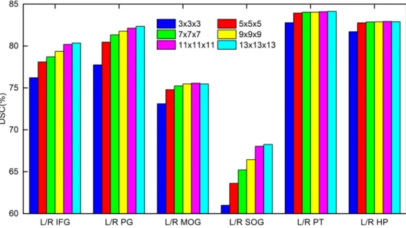
IFG), left and right precentral gyrus (L/R PG), left and right middle orbitofrontal gyrus (L/R MOG), left and right superior occipital gyrus (L/R SOG), left and right putamen (L/R PT), and left and right hippocampus (L/R HP), respectively. The L/R IFG and PG volumes contain about 25 000 voxels, L/R MOG and SOG volumes contain about 10 000 voxels, and L/R PT and HP volumes contain about 5000 voxels. Note that the image resolution of the LONI database is 1×1 ×1 mm3.
To compare the labeling performance with different appear-ance patch size, we vary the patch size from 3×3×3 to 15×15×15 mm3. Figure5shows the DSCs of 12 ROIs using SRF without incorporating the label features. It is clearly seen that, for large ROIs (L/R IFG, PG, MOG, SUG), using the larger appearance patch size leads to better performance. By varying the appearance patch size from 3×3×3 to 15×15×15, the DSCs of L/R IFG, PG, MOG and SOG, respectively, arise from 61.4% to 71.5%, 61.3% to 70.2%, 62.2% to 71.8%, 47.1% to 56.5%, 75.3% to 83.9%, and 77% to 82.6%. When the appearance patch size is larger than 11×11×11, the performance becomes stable. On the other hand, for the small ROIs (L/R PT, HP), stable DSCs have been obtained with patch size 9×9×9. It is worth noting that, when using a large appearance patch size (e.g., 15×15×15), the labeling performances of small ROIs are still kept stable and do not descend, indicating that large appearance patch size is also beneficial for labeling small ROIs.
Similar to the process for the appearance patch size, we also vary the label patch size from 3×3×3 to 13×13×13
in our SAMCF framework. In this experiment, we set the appearance patch size as 11×11×11 mm3, which is proved to
be the optimal in the previous experiment. Figure6shows the DSCs of the 12 ROIs with different label patch size. We can see similar results with those of appearance patch sizes. The larger the patch size is, the better the labeling performance is. Also, a large patch size does not lead to a decrease of labeling performance for small ROIs. To balance performance in ROIs with different volumes, both appearance and label patches with size of 11×11×11 mm3are used to label all ROIs in the
following experiments.
3.A.2.b. The effectiveness of atlas-guided random forest. In evaluation of atlas-guided spatial label context information, we compare the SRF (that does not use spatial label context information) with both the single atlas-guided multi-channel forest (SAMCF) and the multiple atlas-guided multi-channel forest (MAMCF). Additionally, in order to analyze the effect of label information of multiple ROIs, SAMCF (multi-ROI), relative to single ROI of SAMCF [the SAMCF with only single-ROI label features, namely, SAMCF (single ROI)], is also evaluated. Specifically, for SAMCF (single ROI) and SAMCF (multi-ROI), we select 20 subjects as the training images, one subject in the remaining 20 subjects as atlas, and the rest of the 19 subjects as the testing images. For fair comparison, for both SRF and MAMCF (multi-ROI), we use the same 20 training images and also test on the same 19 images as SAMCF (multi-ROI).
TableIlists the mean and standard deviation of DSC on all 54 ROIs for SRF, SAMCF (single ROI), SAMCF (multi-ROI),
TI. The mean and standard deviation of DSCs of 54 ROIs on LONI_LPBA40 dataset, produced by SRF,
SAMCF (single ROI), SAMCF (multi-ROI), and MAMC (multi-ROI), respectively.
Method SRF SAMCF (single ROI) SAMCF (multi-ROI) MAMCF (multi-ROI)
1012 Maet al.: Nonlocal atlas-guided multi-channel forest learning 1012
F. 7. The effectiveness of using atlas-guided spatial label context information in labeling each of 54 ROIs in the LONI_LPBA40 dataset.
and MAMCF (multi-ROI), respectively. It can be seen that the MAMCF (multi-ROI) method achieves the highest measure (81.51%±4.27%). In the meanwhile, SAMCF (multi-ROI) (79.67%±4.35%) also achieves 7.19% increase of the average DSC over SRF (72.48%±4.36%). These results indicate that the atlas-guided spatial label context information is useful to improve the labeling performance. Compared with SAMCF (single ROI) (79.53%±4.53%), SAMCF (multi-ROI) (80.37%±4.32%) achieves better performance, which indicates that multi-ROI label information is more beneficial
to labeling than only using single-ROI label information. Unless explicitly stated, our methods adopt the multi-ROI label information in the following experiments. In Fig.7, we further show the mean DSC of each of 54 ROIs by SRF, SAMCF (single ROI), SAMCF (multi-ROI), and MAMCF (multi-ROI). It is shown that the use of atlas-guided spatial label context information consistently improves the labeling performance in all 54 ROIs. By performing the paired Student’s t-test, compared with SRF, our method SAMCF (single ROI), SAMCF (multi-ROI), and MAMCF (multi-ROI)
TII. The mean and standard deviation of DSCs of 54 ROIs on the
LONI_LPBA40 dataset, produced by SAMCF with 1, 5 and 10 nearest atlas voxels selected in the testing stage.
Method SAMCF (Num=1) SAMCF (Num=5) SAMCF (Num=10)
DSC (%) 80.37±4.32 80.82±4.30 80.98±4.29
obtain statistically significant (p<0.05) improvement on 41, 42, and 51 ROIs, respectively. Over all the ROIs, compared with SRF, SAMCF (single ROI), and SAMCF (multi-ROI), MAMCF (multi-ROI) obtains statistically significant improvements with p-values ofp<0.0001, p=0.0066, and p=0.022, respectively.
In order to further analyze the performance of proposed method in segmentation, we also provide the ROC curve analysis for 8 typical ROIs with relatively small volumes from the LONI_LPBA 40 database,7which are relatively difficult to segment. These eight selected ROIs include left (L) MOG, lateral orbitofrontal gyrus (LOG), gyrus rectus (GR), SOG, cuneus (CN), parahippocampal gyrus (PHG), PT and HP in the left brain. ROI curves of two methods, SRF and MAMCF (multi-ROI), for these eight selected ROIs are shown in Fig.8. In terms of AUC (the area under the ROC curve), for these eight selected ROIs, SRF and MAMCF (multi-ROI), respectively, obtain (0.853, 0.922), (0.82, 0.903), (0.878, 0.91), (0.806, 0.908), (0.776, 0.848), (0.89, 0.928), (0.933, 0.951), and (0.895, 0.918). Compared with SRF, our method [MAMCF (multi-ROI)] obtains much higher AUC over all these eight selected ROIs.
3.A.2.c. Nonlocal strategy in brain labeling. In our method, we adopt the nonlocal strategy to search top K matching label patch with target patch from the aligned atlas for labeling. In the evaluation of nonlocal strategy in brain
T III. The mean and standard deviation of DSCs of 54 ROIs on
LONI_LPBA40 dataset, produced by SRF, SRF+ACM, SRF+HSCCM, and SRF+HMCCM, respectively.
Method SRF SRF+ACM SRF+HSCCM SRF+HMCCM
DSC (%) 72.48±4.36 73.83±4.47 77.11±4.41 77.99±4.38
labeling, we take SAMCF method as example and respectively set the numberKof nearest atlas voxels as one, five, and ten. The mean and standard deviation of DSC by SAMCF with one, five, and ten nearest atlas voxels selected in the testing stage are shown in TableII. It is shown that, when we fuse the label information from ten nearest atlas voxels, SAMCF achieves the highest average DSC as well as the minimum standard deviation (80.98%±4.29%). Its average DSC is 0.61% higher than SAMCF with the use of only one nearest atlas voxel. It is evident that the use of a nonlocal strategy in the testing stage can not only improve the labeling performance but also enhance the robustness. Figure9shows the mean DSC of each of 54 ROIs by SAMCF with a different number of nearest atlas voxels. It is clear that the use of a nonlocal strategy consistently improves the performance in all 54 ROIs.
3.A.2.d. Haar-like multi-ROI context model. Besides, in contrast to HMCCM, we can also consider using the HSCCM for extensive comparison. In Table III, we provide the mean and standard of DSC on all 54 ROIs, produced by SRF, SRF+ACM, SRF+HSCCM, and SRF+HMCCM, respectively. (Note that ACM stands for auto-context model, as mentioned above.) It can be observed that SRF+HMCCM achieves the highest DSC (77.99%±4.38%) over any other methods, followed by SRF+HSCCM (77.11%±4.41%), SRF+ACM (73.83%±4.47%), and SRF (72.48%±4.36%). Both SRF+HMCCM and SRF+HSCCM methods achieve
1014 Maet al.: Nonlocal atlas-guided multi-channel forest learning 1014
F. 10. The effectiveness of using HMCCM in labeling each of 54 ROIs in the LONI_LPBA40 dataset.
6.38% and 5.88% improvement over SRF+ACM, respectively. In contrast, SRF+ACM gains only 1.35% increases over SRF. These results indicate that the extraction of Haar-like features, from the label probability maps, is more effective than the simple extraction of traditional context information, from the sparse voxels of label probability maps. In terms of multi-class context information, the mean DSC of SRF+HMCCM is 0.88% higher than that of SRF+HSCCM, indicating that using the context information from multi-ROI label probability maps is more effective for labeling than using only the single-ROI label context information. The detailed DSC ratios on all 54 ROIs by SRF, SRF+ACM, SRF+HSCCM, and SRF+HMCCM are shown in Fig.10.
3.A.3. Comparison with existing multi-atlas based methods
The second column of Table IV shows the mean and standard deviation of DSC on 54 ROIs by (1) multi-atlas based Majority Voting (MV); (2) two state-of-the-art
TIV. The mean and standard deviation of DSC (%) by MV, nonlocal
PBL, sparse PBL, MAMCF, and MAMCF+HMCCM on LONI_LPBA40 and IXI datasets, respectively. Asterisks in MAMCF and MAMCF+HMCCM rows denote that MAMCF and MAMCF+HMCCM have statistically sig-nificant improvement over MV, nonlocal PBL, sparse PBL, as per paired Student’st-test.
Method LONI_LPBA40 IXI
MV 78.55±4.33 76.64±4.56
Nonlocal PBL 78.58±4.32 75.85±4.70 Sparse PBL 80.21±4.32 77.4±4.52 MAMCF 81.89±4.25a 79.08±4.41a
MAMCF+HMCCM 82.56±4.22a 79.78±4.34a
ap<0.0001.
multi-atlas based labeling methods, i.e., nonlocal PBL (Ref.12) and sparse PBL,13 and (3) the proposed methods, i.e., MAMCF and MAMCF+HMCCM. The average DSC achieved by MV, nonlocal PBL, and sparse PBL for all 54 ROIs are 78.55%±4.33%, 78.58%±4.32% and 80.21% ±4.32%, respectively, which are lower than 81.89%±4.25% achieved by MAMCF and 82.56%±4.22% achieved by MAMCF+HMCCM. This comparison indicates the impor-tance of learning a nonlinear classifier to fuse information from both the target image and the atlas label map. Figure11further compares our methods (MAMCF and MAMCF+HMCCM) with MV, nonlocal PBL and sparse PBL on each of 54 ROIs. In terms of average performance over all the ROIs, compared with MV, nonlocal PBL, and sparse PBL, both MAMCF and MAMCF+HMCCM obtain statistically significant improvements (p<0.0001).
3.A.4. Comparison with existing learning-based methods
F. 11. Comparison of performance of our proposed MAMCF and MAMCF+HMCCM methods and three multi-atlas based labeling methods in labeling
each of 54 ROIs from LONI_LPBA40 dataset. Each green star “*” denotes that MAMCF+HMCCM has significant improvement over all other methods (with
P<0.05) in the particular ROI. Also, a green star in the left of “/” denotes significant improvement on the left ROI, while a green star in the right of “/” denotes significant improvement on the right ROI.
obtain statistically significant improvements (p<0.0001). In addition, compared with our previous method21 (81.35% ±4.35%), both MAMCF and MAMCF+HMCCM achieve the statistically significant improvements with p=0.017 and p=0.011, respectively.
3.B. Experiments on IXI dataset
3.B.1. Data description
We use a subset of 30 images in the IXI dataset, containing manual annotations of 80 structures (excluding cerebrum and brainstem). The size of each image is 256×256×198. Again, the intensity normalization of each brain image is performed by histogram matching before labeling, where the MR brain image of the first subject is used as a template for histogram
T V. The mean and standard deviation of DSC (%) by SRF, SRF+HMCCM, MAMCF, and MAMCF+HMCCM on LONI_LPBA40 and IXI datasets, respectively. Asterisks in MAMCF and MAMCF+HMCCM rows denote that MAMCF and MAMCF+HMCCM have statistically signifi-cant improvement over SRF, SRF+ACM, as per paired Student’st-test.
Method LONI_LPBA40 IXI
SRF 72.48±4.36 72.09±4.98
SRF+ACM 73.83±4.47 74.53±4.49 Previous work 81.35±4.35 — MAMCF 81.89±4.25a 79.08±4.41a
MAMCF+HMCCM 82.56±4.22a 79.78±4.34a
ap<0.0001.
matching. We use leave-one-out cross-validation to evaluate the performance of our method by using 15 images for training and the other 14 images as atlas images in each fold.
3.B.2. Comparison with existing multi-atlas based methods
The third column of TableIVshows the mean and standard deviation of DSC on all 80 ROIs in the IXI dataset by MV, nonlocal, sparse PBL, MAMCF, and MAMCF+HMCCM. It can be observed that our MAMCF+HMCCM (79.78% ±4.34%) and MAMCF (79.08%±4.41%) methods are ranked top, followed by sparse PBL (77.4%±4.52%), MV (76.64% ±4.56%), and nonlocal PBL (75.85%±4.7%). This denotes that our methods consistently outperform the multi-atlas based labeling methods. In terms of average performance over all the ROIs, our MAMCF and MAMCF+HMCCM methods have significant improvement (p<0.0001) over MV, nonlocal PBL, and sparse PBL, respectively. Also, Fig.13shows the detailed DSC on each of 80 ROIs in IXI dataset by MV, nonlocal, sparse PBL, MAMCF, and MAMCF+HMCCM.
3.B.3. Comparison with existing learning-based methods
1016 Maet al.: Nonlocal atlas-guided multi-channel forest learning 1016
F. 12. Comparisons between the proposed MAMCF and MAMCF+HMCCM methods and two other learning-based labeling methods on each of 54 ROIs from LONI_LPBA40 dataset. See Fig.11for description of the green stars.
(79.78%±4.34%) methods outperform other learning based methods, SRF (72.09%±4.98%) and SRF+ACM (74.53% ±4.49%). Figure 14 shows the detailed DSC on each of 80 ROIs in IXI dataset by SRF, SRF+ACM, MAMCF, and
MAMCF+HMCCM. In terms of average performance over all the ROIs, compared to the baseline method SRF, SRF+ACM, MAMCF, and MAMCF+HMCCM obtain statistically signif-icant improvements (p<0.0001).
F. 13. Comparisons between the proposed MAMCF and MAMCF+HMCCM methods and three multi-atlas based labeling methods on each of 80 ROIs in
F. 14. Comparisons between the proposed MAMCF and MAMCF+HMCCM methods and two other learning-based labeling methods on each of 80 ROIs in IXI dataset. See Fig.11for description of the green stars.
4. DISCUSSION AND CONCLUSIONS
Learning-based methods and multi-atlas based methods have been widely applied to a large variety of medical image segmentation problems. In this work, we focus on the development of a new labeling method, which can effectively combine the advantages of both multi-atlas based labeling methods and learning-based labeling methods, applied to automated human brain labeling. Multi-atlas based label-ing methods take advantage of similarities between image intensity patches to propagate labels from warped atlases to the target image. These methods allow the selection of few good candidates (i.e., the most similar patches) for label estimation. However, the definition of patch-based similarity is often handcrafted which may not be effective for labeling all types of brain structures. In contrast to these methods, the learning-based labeling methods aim to learn the mapping between image intensity patches and the corresponding labels. In the testing stage, these methods label a target image based on only the appearance information, without utilizing the label information from the warped atlases. In our method, label features are also extracted from the wrapped atlas and then combined with local appearance features of the target image as input to learn the nonlinear mapping between image intensity patches and their corresponding labels. In this way, our method considersnot onlyimage appearance information
but also the label information of warped atlases during the learning procedure, which eventually improves the labeling performance compared to the conventional learning-based methods. In order to effectively and efficiently use atlas label information, a classifier is learned for each atlas based on its label map. In the testing stage, the labeling results from all atlases are fused for final labeling. Furthermore, the HMCCM is also proposed to enhance the structural and label context information of the target image. Specifically, we use Haar-like features to iteratively extract multi-scale label context information from the tentatively estimated multi-ROI label probability maps of the target image, which gradually improves the labeling results.
1018 Maet al.: Nonlocal atlas-guided multi-channel forest learning 1018
learned based on a set of training images, thus not suffering this overfitting problem. However, it has to be indicated that their method is faster, due to the reduced time in atlas registration (only once), while our method needs to perform image registration between each atlas and the target image. Compared to the ACM proposed by Tu and Bai,19 our
presented HMCCM extracts Haar-like features, which contain richer contexture information. Experiment results confirm the superiority of our HMCCM model over the conventional ACM.
The experiments on two public T1-weighted MR images datasets (LONI_LBPA40 and IXI) have shown that the proposed method can perform high-quality labeling of human brain MR images. To capture appearance information around each voxel, the patch size is important. If the patch size is too small, useful information may be lost. On the other hand, if the patch size is too large, noisy and useless information could be included. In our proposed method, due to the built-in feature selection mechanism in random forests, the useful features in the patch can be preserved while the useless information is filtered out. As shown in Figs. 5 and 6, although a large patch size is used for both intensity and label images, the performance of our method does not descend, thanks to the feature selection mechanism in random forests.
Our method utilizes the label information from multiple warped atlases for classifier training, which shows a better performance than the same information from a single atlas. Table I compares the results obtained by label information of a single atlas (SAMCF) and multiple atlases (MAMCF), respectively, which show that the latter could lead to a better performance. Meanwhile, as shown in Table II, the use of few good label patch candidates from a single atlas, i.e., SAMCF (number=10), can also improve the performance. In our method, the performance can be further boosted by HMCCM.
In order to efficiently make use of label information of multiple atlases, we learn a classifier for each atlas. In the testing stage, we fuse the labeling results from all the atlases by using major voting. However, since some atlases can be highly different from the target image, using their label information could potentially lead to wrong labeling results. To predict the label of each voxel, only the results from the reliable atlas-specific classifiers should be considered for obtaining the final labeling result. Thus, one of our future works is to develop a method to evaluate the reliability of each atlas-specific classifier and then select only the reliable results for fusion. Also, to increase the computational efficiency of proposed method, the nonrigid registration method can be replaced with a linear registration method, and the corresponding performance will be evaluated. Finally, our method should be also tested on segmenting some important subcortical structures such as hippocampus.
Finally, multi-atlas based and learning-based methods have been heavily used in many other segmentation problems, such as CT head and neck segmentation29and tooth segmentation.30
In our future work, we also plan to evaluate our method in those applications.
ACKNOWLEDGMENTS
This work was supported in part by NIH Grant Nos. EB006733, EB008374, EB009634, MH100217, AG041721, and AG042599, the National Natural Science Foundation of China (Nos. 61174126, 61222301, and 61473190), the Fok Ying Tung Education Foundation (No. 141059), and the Fundamental Research Funds for the Central Universities (No. HIT.BRETIV.201303).
APPENDIX: LOCAL APPEARANCE FEATURES Given a sampled voxel x, we extract the following local appearance features from the (training) target imageH:
1. Patch intensities within a 7×7×7 neighborhoodC7,7,7,
H(x1),x1∈C7,7,7(x).
2. Outputs of the FODs,
H(x+u1)−H(x−u1).
3. Outputs of the SODs,
H(x+u1)+H(x−u1)−2H(x).
4. Outputs of 3D hyperplan filters,
Ψ1∗(H(C3,3,1(x+u2))−H(C3,3,1(x−u2))).
5. Outputs of 3D Sobel filters,
Ψ2∗(H(C3,3,1(x+u2))−H(C3,3,1(x−u2))).
6. Outputs of Laplacian filters,
x1∈Op(x)
(H(x1)−H(x)).
7. Outputs of range difference filters,
max x1∈Op(x)(
H(x1))− min
x1∈Op(x)(
H(x1)).
8. The random 3D Haar-like features,
w1
x3∈Ca,b,c(x1)
H(x3)
−w2
x4∈Ca′,b′,c′(x2)
H(x4),x1,x2∈C11,11,11(x),
whereCa,b,c(x)denotes the cube centered atxwith size ofa ×b×c,u1=(rcosθsinφ,rsinθcosφ,rcosφ)andu2=(0,0,1)
are offset vectors,ris the length ofu1,θandφare two rotation
angles ofu1,Ψ1= 1 1 1
1 1 1 1 1 1
andΨ2= 1 2 1
2 3 2 1 2 1
are filter functions,
* denotes convolution operation,Op(x)denotes the set ofp
-neighborhood voxels ofx, andw1andw2are weight scalars.
Specifically, FODs and SODs detect intensity change along a line segment. In this implementation, we user∈{1,2,3},
the difference between maximal and minimal values in a given neighborhood of each voxel. In this implementation, we set the size of neighborhoodp∈{7,19,27}. The random 3D Haar-like features describe rich texture information of appearance image by computing the sum value of intensities in the cube, or difference of the sum values between cubes of different sizes located at different positions. In this implementation, for each Haar feature, we randomly selecta,b,c,a′,b′,c′from
{1,3,5}, (w1,w2) from {(1,0),(1,−1)}, and the positionsx1 andx2 of
two Haar cubes within the local neighborhood 7×7×7.
a)Author to whom correspondence should be addressed. Electronic mail: [email protected]
1S. Zhang, Y. Zhan, M. Dewan, J. Huang, D. N. Metaxas, and X. S. Zhou, “Towards robust and effective shape modeling: Sparse shape composition,”
Med. Image Anal.16, 265–277 (2012).
2C. Fennema-Notestine, D. J. Hagler, L. K. McEvoy, A. S. Fleisher, E. H. Wu, D. S. Karow, and A. M. Dale, “Structural MRI biomarkers for preclin-ical and mild Alzheimer’s disease,”Hum. Brain Mapp.30, 3238–3253 (2009).
3R. Westerhausen, E. Luders, K. Specht, S. H. Ofte, A. W. Toga, P. M. Thomp-son, T. Helland, and K. Hugdahl, “Structural and functional reorganization of the corpus callosum between the age of 6 and 8 years,”Cereb. Cortex21, 1012–1017 (2010).
4G. Wu, Q. Wang, D. Zhang, F. Nie, H. Huang, and D. Shen, “A generative probability model of joint label fusion for multi-atlas based brain segmen-tation,”Med. Image Anal.18, 881–890 (2014).
5L. Wang, Y. Gao, F. Shi, G. Li, J. H. Gilmore, W. Lin, and D. Shen, “Links: Learning-based multi-source integration framework for segmentation of infant brain images,”NeuroImage108, 160–172 (2015).
6H. Wang, J. W. Suh, S. R. Das, J. B. Pluta, C. Craige, and P. Yushkevich, “Multi-atlas segmentation with joint label fusion,”IEEE Trans. Pattern Anal. Mach. Intell.35, 611–623 (2013).
7G. Sanroma, G. Wu, Y. Gao, and D. Shen, “Learning to rank atlases for multiple-atlas segmentation,”IEEE Trans. Med. Imaging33, 1939–1953 (2014).
8T. Tong, R. Wolz, P. Coupé, J. V. Hajnal, D. Rueckert, and The Alzheimer’s Disease Neuroimaging Initiative, “Segmentation of MR images via discrim-inative dictionary learning and sparse coding: Application to hippocampus labeling,”NeuroImage76, 11–23 (2013).
9Y. Gao, S. Liao, and D. Shen, “Prostate segmentation by sparse representa-tion based classificarepresenta-tion,”Med. Phys.39, 6372–6387 (2012).
10G. Wu, Q. Wang, H. Jia, and D. Shen, “Feature-based groupwise registration by hierarchical anatomical correspondence detection,”Hum. Brain Mapp.
33, 253–271 (2012).
11T. Vercauteren, X. Pennec, A. Perchant, and N. Ayache, “Diffeomorphic demons: Efficient non-parametric image registration,” NeuroImage 45, S61–S72 (2009).
12P. Coupé, J. V. Manjón, V. Fonov, J. Pruessner, M. Robles, and D. L. Collins, “Patch-based segmentation using expert priors: Application to hippocampus and ventricle segmentation,”NeuroImage54, 940–954 (2011).
13G. Wu, Q. Wang, D. Zhang, and D. Shen, “Robust patch-based multi-atlas labeling by joint sparsity regularization,” in MICCAI Workshop STMI (Springer, Berlin Heidelberg, 2012).
14V. N. Vapnik and V. Vapnik,Statistical Learning Theory(Wiley, New York, NY, 1998), Vol. 1.
15Y. Freund and R. E. Schapire, “A desicion-theoretic generalization of on-line learning and an application to boosting,” inComputational Learning Theory (Springer, Berlin Heidelberg, 1995), pp. 23–37.
16L. Breiman, “Random forests,”Mach. Learn.45, 5–32 (2001).
17V. A. Magnotta, D. Heckel, N. C. Andreasen, T. Cizadlo, P. W. Corson, J. C. Ehrhardt, and W. T. Yuh, “Measurement of brain structures with artificial neural networks: Two-and three-dimensional applications 1,”Radiology
211, 781–790 (1999).
18D. Zikic, B. Glocker, and A. Criminisi, “Atlas encoding by randomized forests for efficient label propagation,” inMedical Image Computing and Computer-Assisted Intervention–MICCAI 2013(Springer, Berlin Heidel-berg, 2013), pp. 66–73.
19Z. Tu and X. Bai, “Auto-context and its application to high-level vision tasks and 3D brain image segmentation,”IEEE Trans. Pattern Anal. Mach. Intell.
32, 1744–1757 (2010).
20Y. Hao, T. Wang, X. Zhang, Y. Duan, C. Yu, T. Jiang, and Y. Fan, “Local label learning (LLL) for subcortical structure segmentation: Application to hippocampus segmentation,”Hum. Brain Mapp.35, 2674–2697 (2014). 21G. Ma, Y. Gao, G. Wu, L. Wu, and D. Shen, “Atlas-guided multi-channel
for-est learning for human brain labeling,” inMedical Computer Vision: Algo-rithms for Big Data(Springer, International Publishing, 2014), pp. 97–104. 22M. Seyedhosseini and T. Tasdizen, “Multi-class multi-scale series contex-tual model for image segmentation,” IEEE Trans. Image Process. 22, 4486–4496 (2013).
23M. Kim, G. Wu, W. Li, L. Wang, Y.-D. Son, Z.-H. Cho, and D. Shen, “Auto-matic hippocampus segmentation of 7.0 Tesla MR images by combining multiple atlases and auto-context models,”NeuroImage83, 335–345 (2013). 24D. W. Shattuck, M. Mirza, V. Adisetiyo, C. Hojatkashani, G. Salamon, K. L. Narr, R. A. Poldrack, R. M. Bilder, and A. W. Toga, “Construction of a 3D probabilistic atlas of human cortical structures,”NeuroImage39, 1064–1080 (2008).
25F. Shi, L. Wang, Y. Dai, J. H. Gilmore, W. Lin, and D. Shen, “Label: Pediatric brain extraction using learning-based meta-algorithm,”NeuroImage 62, 1975–1986 (2012).
26N. J. Tustison, B. B. Avants, P. Cook, Y. Zheng, A. Egan, P. Yushkevich, and J. C. Gee, “N4ITK: Improved N3 bias correction,”IEEE Trans. Med. Imaging29, 1310–1320 (2010).
27S. M. Smith, M. Jenkinson, M. W. Woolrich, C. F. Beckmann, T. E. Behrens, H. Johansen-Berg, P. R. Bannister, M. De Luca, I. Drobnjak, D. E. Flitney, and R. K. Niazy, “Advances in functional and structural MR image analysis and implementation as FSL,”NeuroImage23, S208–S219 (2004). 28Http://www.loni.ucla.edu/Atlases/LPBA40.
29K. D. Fritscher, M. Peroni, P. Zaffino, M. F. Spadea, R. Schubert, and G. Sharp, “Automatic segmentation of head and neck CT images for radio-therapy treatment planning using multiple atlases, statistical appearance models, and geodesic active contours,”Med. Phys.41, 051910 (11pp.) (2014).