0e8d288eb0ab73a1786db01a00c97f2257d36a34.pdf

(1)

THE INFRARED SPECTRAL PROPERTIES OF MAGELLANIC CARBON STARS

G. C. Sloan1,2, K. E. Kraemer3, I. McDonald4, M. A. T. Groenewegen5, P. R. Wood6, A. A. Zijlstra4, E. Lagadec7, M. L. Boyer8,9, F. Kemper10, M. Matsuura11, R. Sahai12, B. A. Sargent13, S. Srinivasan10,

J. Th. van Loon14, and K. Volk15

1

Cornell Center for Astrophysics & Planetary Science, Cornell Univ., Ithaca, NY 14853-6801, USA;[email protected]

2

Department of Physics and Astronomy, University of North Carolina, Chapel Hill, NC 27599-3255, USA

3

Institute for Scientiﬁc Research, Boston College, 140 Commonwealth Avenue, Chestnut Hill, MA 02467, USA

4

Jodrell Bank Centre for Astrophysics, Univ. of Manchester, Manchester M13 9PL, UK

5

Koninklijke Sterrenwacht van België, Ringlaan 3, B-1180 Brussels, Belgium

6

Research School of Astronomy and Astrophysics, Australian National University, Canberra, ACT 2611, Australia

7

Observatoire de la Côte d’Azur, F-06300, Nice, France

8

CRESST and Observational Cosmology Lab, Code 665, NASA Goddard Space Flight Center, Greenbelt, MD, 20771, USA

9

Department of Astronomy, University of Maryland, College Park, MD 20742, USA

10

Academia Sinica, Institute of Astronomy and Astrophysics, 11F Astronomy-Mathematics Building, NTU/AS, No. 1, Sec. 4, Roosevelt Rd., Taipei 10617, Taiwan, R.O.C.

11_{School of Physics and Astronomy, Cardiff University, Queen’s Buildings, The Parade, Cardiff, CF24 3AA, UK} 12

Jet Propulsion Laboratory, California Institute of Technology, MS 183-900, Pasadena, CA 91109, USA

13_{Center for Imaging Science and Laboratory for Multiwavelength Astrophysics, Rochester Institute of Technology,}

54 Lomb Memorial Drive, Rochester, NY 14623, USA

14

Lennard Jones Laboratories, Keele University, Staffordshire ST5 5BG, UK

15

Space Telescope Science Institute, 3700 San Martin Dr., Baltimore, MD 21218, USA Received 2015 December 23; revised 2016 April 8; accepted 2016 April 15; published 2016 July 18

ABSTRACT

The Infrared Spectrograph on the Spitzer Space Telescopeobserved 184 carbon stars in the Magellanic Clouds. This sample reveals that the dust-production rate(DPR)from carbon stars generally increases with the pulsation period of the star. The composition of the dust grains follows two condensation sequences, with more SiC condensing before amorphous carbon in metal-rich stars, and the order reversed in metal-poor stars. MgS dust condenses in optically thicker dust shells, and its condensation is delayed in more metal-poor stars. Metal-poor carbon stars also tend to have stronger absorption from C2H2at 7.5μm. The relation between DPR and pulsation period shows signiﬁcant apparent scatter, which results from the initial mass of the star, with more massive stars occupying a sequence parallel to lower-mass stars, but shifted to longer periods. Accounting for differences in the mass distribution between the carbon stars observed in the Small and Large Magellanic Clouds reveals a hint of a subtle decrease in the DPR at lower metallicities, but it is not statistically signiﬁcant. The most deeply embedded carbon stars have lower variability amplitudes and show SiC in absorption. In some cases they have bluer colors at shorter wavelengths, suggesting that the central star is becoming visible. These deeply embedded stars may be evolving off of the asymptotic giant branch and/or they may have non-spherical dust geometries.

Key words:circumstellar matter –infrared: stars –stars: AGB and post-AGB–stars: carbon

Supporting material:machine-readable tables

1. INTRODUCTION

Intermediate-mass stars contribute to the chemical evolution of galaxies when they shed their envelopes and seed their environments with freshly condensed dust and the products of nuclear fusion from their cores. The sensitivity of the Infrared Spectrograph (IRS; Houck et al. 2004) on the Spitzer Space Telescope (Werner et al. 2004) made it possible to observe many mass-losing stars in nearby galaxies like the Large and Small Magellanic Clouds(LMC and SMC). These stars are at known distances, and they probe different metallicities. While the metallicity distribution functions are broad enough to overlap and depend on age, for statistical treatment of large samples it is safe to claim that the LMC is more metal-poor than the Galaxy, and the SMC is more metal-poor still. As an example, Piatti & Giesler(2013)ﬁnd that in the LMC,[Fe/H] increased from∼−0.7 to∼−0.3 from 5 to 1 Gyr ago, compared to ∼−1.2 to ∼−0.6 over the same time interval in the SMC (Piatti2012).

Carbon stars dominated the spectral samples of evolved stars observed early in the Spitzer mission. Sloan et al. (2006)

examined carbon stars in the SMC while Zijlstra et al.(2006)

considered the LMC. Matsuura et al. (2006) studied the molecular absorption in these samples, and other studies followed(Buchanan et al.2006; Lagadec et al.2007; Leisenring et al. 2008; Sloan et al. 2008). Further observing programs added considerably to the spectral sample of carbon stars in both galaxies, including two programs which added fainter carbon stars to the samples in the LMC (Kemper et al. 2010)

and SMC(Program 50240).

These earlier efforts led to theﬁnding that the amount of dust observed around carbon stars does not show a strong dependence on metallicity (Sloan et al. 2008). Carbon stars result from the dredge-up of freshly fused carbon from the cores of stars as they burn He in thermal pulses while on the asymptotic giant branch (AGB). The formation of CO leaves only carbon or oxygen available to form other molecules and condense into dust so that when the C/O ratio exceeds unity, the gas and dust shift from an O-rich to a C-rich chemistry. Matsuura et al.(2005)noted that because dredged-up material on the AGB is dominated by carbon in most stars, the amount

(2)

of free carbon left after the formation of CO should actually

increase in more metal-poor stars. Sloan et al. (2012)

accounted for the changing oxygen abundances at lower metallicity and reached a similar conclusion. Thus, the question is not one of why the amount of carbon-rich dust is not

decliningas metallicity drops, but why is it not increasing. The infrared spectrographic studies of Magellanic carbon stars have revealed several dependencies on metallicity. In more metal-poor samples, the SiC dust emission feature at

∼11.3μm weakens, the molecular absorption bands from C2H2 at 7.5 and 13.7μm grow stronger, and the appearance of MgS dust is more delayed.

This work builds on the earlier works by adding the rest of the IRS observations and comparing the samples as a whole. Section 2 describes the samples of carbon stars in the Magellanic Clouds and the Galaxy and the spectroscopic and photometric data. Section 3 describes the data analysis, and Section 4 presents the results. In Section 5, we discuss the issues raised, and in Section 6, summarize our ﬁndings. Appendix A presents useful relations between infrared ﬁlter sets and colors for carbon stars. AppendicesB and Cpresent new periods for several sources based on the analysis of multi-epoch photometry in the near-IR and mid-IR, respectively.

2. OBSERVATIONS

2.1. Samples and Targets

Table1lists the 144 objects in the LMC and 40 in the SMC observed with the IRS and identiﬁed as carbon stars. Our objective was to build a sample including all of the carbon-rich AGB stars observed by the IRS while excluding post-AGB objects. Our selection criteria are based on the infrared (IR) spectral classiﬁcation of Kraemer et al.(2002, see Section2.5

below). Generally, spectra are considered carbon-rich if they show SiC dust emission at ∼11.3μm or the acetylene absorption bands at 7.5 and/or 13.7μm. The 26–30μm feature attributed to MgS dust appears in many of the spectra and helps to conﬁrm their carbon-rich nature.

Goebel & Moseley(1985)identiﬁed MgS dust as the carrier of the 26–30μm feature, but some doubt has been cast on that identiﬁcation due to abundance constraints (e.g., Zhang

et al. 2009). Sloan et al. (2014) examined these and other concerns about MgS and concluded that it remains a strong candidate for the carrier of the feature. Section5.4investigates this issue, but in the meantime, we will refer to this feature as the MgS feature for convenience.

We excluded objects if their spectra peak at wavelengths above ∼20μm(inF_ν units), because for carbon-rich sources, that indicates that they have evolved past the AGB. These excluded objects are part of the carbon-rich post-AGB sample studied by Sloan et al.(2014).

Two other classes of post-AGB objects have warmer spectral energy distributions(SEDs)peaking shortward of∼20μm and are also excluded. RCrB stars have smooth spectra showing only emission from amorphous carbon dust and no other signiﬁcant spectral features. Kraemer et al.(2005)examined two in the SMC, but the IRS sample contains additional R CrB stars (G. C. Clayton et al. 2016, in preparation). The other class of warm post-AGB objects includes two sources showing absorp-tion bands from aliphatic hydrocarbons16: SMPLMC011 (Bernard-Salas et al. 2006), and MSXSMC029 (Kraemer et al.2006).

A variety of Spitzerobserving programs contributed to the present sample of carbon stars (see Table 2). Each program comes with its own selection criteria and biases, which means that the present sample is neither uniform nor complete. However, thanks to the efforts of the designers of all the previous programs, the present sample probes carbon stars spanning a wide range of luminosities, colors, and evolutionary stages.

The ﬁrst two programs listed in Table 2 were developed prior to launch as part of the guaranteed-time observations. Both sampled a variety of evolved stars, with Program 200 focused on supergiants and AGB stars identiﬁed as variable stars in the optical and near-IR in both the SMC and LMC. Program 1094 covered a range of post-main-sequence evolu-tionary stages in the LMC(and the Galaxy).

The next four programs were Guest Observer(GO)programs in Cycle 2 of the mission. Program 3277 started with the mid-Table 1

TheSpitzerSample of Magellanic Carbon Stars

Target Alias R.A. decl. Position Period Period Program

(J2000) Reference (days) Referencea Identiﬁerb

GM 780 L 8.905255 −73.165604 2MASS 611 OGLE 3505

MSX SMC 091 L 9.236293 −72.421547 2MASS K K 3277

MSX SMC 062 L 10.670455 −72.951599 2MASS 550 OGLE 3277

2MASS J004326 L 10.860405 −73.445366 2MASS 330 R05 50240

GB S06 MSX SMC 060 11.668442 −73.279793 2MASS 435 OGLE 3277

Notes.

a

OGLE—Soszyński et al.(2009,2011, Optical Gravitational Lensing Experiment), GO7—Groenewegen et al.(2007), G09—Groenewegen et al.(2009), K10— Kamath et al.(2010), N00—Nishida et al.(2000), R05—Raimondo et al.(2005), S06—Sloan et al.(2006), W89—Whitelock et al.(1989), W03—Whitelock et al.

(2003), Z06—Zijlstra et al.(2006); AppendicesBandC—the appendices in this paper.

b

See Table2.

(This table is available in its entirety in machine-readable form.)

16_{I.e., non-aromatic species such as C2H6, longer chains, and other similar}

(3)

IR sources in the SMC identiﬁed by the Mid-course Space Experiment (MSX; Price et al. 2001) to generate a sample spanning color–color space in the near- and mid-IR. Program 3426 sampled a randomly chosen subset of the brightest 150 sources in the LMC. Program 3505 identiﬁed AGB stars in several previous infrared surveys with the help of near-IR color–magnitude diagrams(CMDs). It covered both the LMC and SMC. Program 3591 extended Program 1094 to a larger sample in the LMC.

More programs followed later in the Spitzer mission. Program 37088 concentrated on heavily embedded and thus more evolved stars in the LMC. Program 40650 targeted about 300 candidate young stellar objects (YSOs) in the LMC, as well as several sources described as extremely red objects (EROs) and subsequently identiﬁed as deeply embedded carbon stars(Gruendl et al.2008). The latter group is included in our sample. Program 40519 expanded on all previous programs studying the LMC by observing about 200 targets covering undersampled regions of color–color and color– magnitude space. It included evolved stars and YSOs, relied on the mid-IR photometry from the SAGE survey of the LMC (Surveying the Agents of Galactic Evolution; Meixner et al. 2006), and is known as SAGE-Spec. This program added a number of faint carbon-rich targets to the sample. Program 50240 expanded the targets observed in the SMC in a similar manner. Finally, Program 50338 concentrated on post-AGB candidates in the LMC.

2.2. Adopted Distances

The known distances to the LMC and SMC enable us to study the total luminosities of the stars in our sample. We adopt distance moduli for the LMC and SMC of 18.5 and 18.9, respectively. Measurements of the distance modulus to the LMC cluster around our adopted value. The review by Feast (2013)leads to 18.50; another good example of a recent result is 18.49±0.05 (Pietrzyński et al. 2013). Similarly, our adopted distance modulus to the SMC is close to the mean value reported by Rubele et al. (2015), 18.91±0.02. The distances to these galaxies are only important to our determinations of absolute bolometric magnitudes, and because these have uncertainties larger than 0.1 mag, we are not concerned with precision in the distance modulus to further signiﬁcantﬁgures.

The SMC has a complicated structure, with considerable depth along the line of sight(Gardiner & Hawkins1991). Most of the stars reside in the Bar region, where the mean distance modulus to different regions can vary from ∼18.85 to 19.02

(Rubele et al. 2015). Typical depths in this region are only 2–3kpc (Δ(m−M)0.1), but in the extended Wing region to the east, Nidever et al.(2013)report depths up to∼20kpc (Δ(m−M)0.8). Rubele et al. (2015) ﬁnd mean distance moduli in the eastern regions between∼18.65 and 18.8. Most of the targets are in the Bar, and we will assume they are at our canonical distance modulus(18.9).

We have several targets in the cluster NGC419, which is in the direction of the SMC. Glatt et al. (2008) give a distance modulus of 18.50, the same as for the LMC and about 10 kpc in front of the SMC. They describe how the model which best

ﬁts the optical CMD gives (m−M)o=18.75, while other models give values of 18.60 and 18.94. It is unclear what justiﬁes the reported value of 18.50, and as discussed below, a value of 18.90 is more consistent with the IR data (see Section4.3).

2.3. IRS Observations

The IRS observed the majority of the sources in the standard low-resolution nod sequence, most of them with both the Short-Low (SL) and Long-Low (LL) modules. SL and LL provide spectral coverage at 5–14μm and 14–37μm, respectively, with a resolution(λ/Δλ)of∼80–120. Some of the fainter sources were observed only in SL. Generally, sources were observed in each of the two SL apertures, providingﬁrst- and second-order spectra, then the two LL apertures. Each source was observed in two nod positions in each aperture. Thus a full low-resolution spectrum requires eight pointings.

The carbon-rich EROs observed by Gruendl et al. (2008)

used the SL module, along with Short-High (SH) and Long-High(LH), which cover 10–19 and 19–36μm, respectively, at a resolution of∼300.

The reduction and calibration of the low-resolution spectra followed the standard Cornell algorithm(see Sloan et al.2015a, for a more detailed description). The Cornell processing begins with theflatfielded images provided by version S18.18 of the pipeline at theSpitzerScience Center. Bad pixels in each image are identified and replaced with values based on their neighbors. All images for a given nod position are averaged, then a suitable background image is subtracted from the target image. In SL, the default is an aperture differerence, where the background for a given target is the image with the target in the other aperture, while in LL, the default is a nod difference, with the target in the same aperture, but the other nod. In some cases, the design of the observation or structure or other sources in the background forced a change from the default. Table 2

SpectroscopicSpitzerPrograms that Observed Magellanic Carbon Stars

Program ID Project Leaders Description

200 J.R.Houck & G.C.Sloan Evolved stars in the LMC and SMC

1094 F.Kemper AGB evolution in the LMC(and Galaxy)

3277 M.P.Egan & G.C.Sloan MSX-based sample in the SMC

3426 J.H.Kastner & C.L.Buchanan Bright infrared sources in the LMC

3505 P.R.Wood & A.A.Zijlstra AGB stars in the LMC and SMC

3591 F.Kemper AGB evolution in the LMC

37088 R.Sahai Embedded carbon stars in the LMC

40650 L.W.Looney & R.A.Gruendl YSOs and red sources in the LMC

40519 A.G.G.M.Tielens & F.Kemper Extended the IRS sample in the LMC

50240 G.C.Sloan & K.E.Kraemer Extended the IRS sample in the SMC

(4)

We deviated from the reduction sequence described by Sloan et al. (2015a) by using an optimal-extraction algorithm to extract spectra from the images(Lebouteiller et al.2010). This method ﬁts a supersampled point-spread function(PSF)to the spatial proﬁle in each row of the spectral image and can improve the signal-to-noise ratio (S/N) up to 80%. It proved essential to generating usable spectra for the faintest sources in our sample. However, the method only works for point sources. For extended or mispointed objects, we used the default extraction algorithm which simply sums data in each wavelength element with no weighting.

Our pipeline continues with the standard step of combining spectra from the two nods and comparing the data to identify and reject spikes or divots which had survived the cleaning process. Spectral segments are then stitched together, shifting spectra upwards multiplicatively to the presumably best-centered segment. Finally, extraneous data are removed from the ends of each segment.

Several previous papers on Magellanic carbon stars used the above algorithm, but without the optimal-extraction method which came later (Sloan et al. 2006; Zijlstra et al. 2006; Lagadec et al.2007; Leisenring et al.2008; Sloan et al.2008; Kemper et al. 2010). The optimal extraction has generally improved the quality of the spectra.

2.4. Photometric Data

For all of our targets, we have constructed SEDs based on multi-epoch photometry in the optical, near-IR, and mid-IR.

The mid-IR data come from the SAGE survey of the LMC (Meixner et al.2006)and the SAGE-SMC survey for the SMC (Gordon et al. 2011), which incorporates the S3MC survey (Spitzer Survey of the SMC; Bolatto et al.2007). The SAGE surveys give two epochs, spaced approximately three months apart, for the Infrared Array Camera (IRAC) and the Multi-Imaging Photometer for Spitzer (MIPS). The S3MC survey provides one additional epoch in the core of the SMC. We use all four IRACﬁlters at 3.6, 4.5, 5.8, and 8.0μm and the MIPS 24μm ﬁlter. The SAGE-VAR survey adds four epochs from the WarmSpitzerMission at 3.6 and 4.5μm for portions of the LMC and SMC (Riebel et al. 2015). We found matches with the SAGE-VAR survey for 61 of our carbon stars in the LMC and 26 in the SMC.

We also used additional epochs at 3.4 and 4.6μm from the

Wide-ﬁeld Infrared Survey Experiment (WISE; Wright et al. 2010) and theNEOWISE reactivation mission (Mainzer et al. 2014).17For allWISEdata, we utilized the multi-epoch data tables and collapsed them to one epoch approximately every six months. The publicly available data typically give us four epochs, two in 2010 and two in 2014.

Applying the color corrections derived for carbon stars in AppendixAallows us to convertW1(3.4μm)to[3.6]andW2

(4.6μm) to [4.5]. The combination of the SAGE surveys, including SAGE-VAR, and the WISEdata can give us 10 or more epochs at 3.6 and 4.5μm for some of the stars in our sample.

The WISE survey is less sensitive and has lower angular resolution than the SAGE data, forcing us to reject some questionable data. We rejected bothW1andW2for NGC419

LE35 and MIR1 due to crowding. For IRAS05026 and IRAS05042, the multi-epoch data indicated a detection at W1, but theWISEimages of theﬁeld showed nothing, even though the sources could be seen in W2. The W1–W2 colors were inconsistent with the SAGE data, so we rejected the W1data but keptW2.

Near-IR photometry comes from the 2MASS survey, and the deeper 2MASS-6X survey provides a second epoch atJ,H, and

Ks(Cutri et al.2012; Skrutskie et al.2006). Additional epochs come from the Deep Near-IR Survey of the Southern Sky (DENIS) atJ and Ks (Cioni et al. 2000) and the IR Survey Facility(IRSF)atJ,H, and Ks (Kato et al.2007).

In the optical, we relied on the Magellanic Clouds Photometric Survey(MCPS)atU,B,V, and I(Zaritsky et al.

2002, 2004). DENIS adds data at I. Additional mean magnitudes atV and I in the LMC come from the OGLE-III Shallow Survey (Ulaczyk et al. 2013). Where possible, we replaced the V and I data with mean magnitudes from the OGLE-III surveys of the Magellanic Clouds, which also give pulsation periods and amplitudes(Soszyński et al.2009,2011). We searched for matches to the IRS sources ﬁrst with the SAGE surveys, using positions estimated from the pointing of the IRS. The optimal extraction algorithm estimates the position of a source along a given slit (i.e., in the cross-dispersion direction). For most observations, the nearly perpendicular orientation of the SL and LL slits helps to constrain the position of the source, despite the widths of the slits(∼3 6 and 10 6, respectively). Where possible, we used matches to IRAC to update the initial IRS-based coordinates, then searched for 2MASS counterparts, again updating positions where possible, and then searched the other catalogs. The positions in Table1 are the result.

The median offset from the estimated IRS position to IRAC is 0 37, consistent with a typical IRS pointing error of 0 4. The median offset between the IRAC and 2MASS positions is 0 20. Comparing positions in the IRAC and MIPS catalogs, weﬁnd a median offset of 0 20.

For the most embedded sources, the expected photometry in the near-IR and at 3.6μm is near or below the detection limit, making it possible to mismatch the photometry to blue sources close to the expected positions of our carbon stars. We examined the environments of the most embedded sources, searching for targets within 1′to estimate the source density. For IRAC, the source densities are 1.1–4.8×10−3, and for 2MASS-6X, they are higher, 7.0–8.2×10−3. Our maximum search radius in the LMC was 1 25, which gives a searchﬁeld of 4.9 square arcsec and makes the odds of a mismatch for a given source 0.5%–2.4%. For 2MASS-6X, the odds of a mismatch are 3.4%–4.0% for a given source. Thus, mismatches are unlikely.

However, the above calculations were for ﬁeld stars. For stars in clusters, we compared our near-IR results to the photometry reported by van Loon et al. (2005), and we used these data to replace the J magnitude of one source, NGC1978 MIR1.

Tables 3 and 4 present the resulting photometry. For each photometricfilter, the magnitude is a mean magnitude, and the uncertainty is the standard deviation of the data. When only one epoch of data in a given filter was available, we left the reported uncertainty undefined. While we can have over ten epochs at 3.6 and 4.5μm, at longer wavelengths we are limited

17

(5)

to three epochs in the heart of the SMC and two epochs in the LMC and the outskirts of the SMC.

2.5. Galactic Comparison Spectra

We also consider a Galactic control sample using spectra from the Short-Wavelength Spectrometer (SWS; de Graauw et al. 1996)on the Infrared Space Observatory(ISO; Kessler et al.1996). Leisenring et al.(2008)presented the original list of 34 carbon stars used in earlier comparisons to Magellanic samples. The present sample includes eight additional objects, for a total of 42.

The comparison SWS sample was chosen from spectra classified as carbon stars by Kraemer et al. (2002). Their classification scheme assigns spectra to groups based on the overall shape of the spectrum, with naked stars in Group 1, stellar spectra showing some dust emission in Group 2, spectra dominated by warm dust in Group 3, and spectra dominated by cold dust(so that the spectrum peaks past∼20μm)in Groups 4 and 5. Spectra are assigned to subgroups based on the dominant features in the spectra. The carbon stars are those with the following classifications: 1.NC (naked star with carbon-rich molecular absorption bands), 2.CE and 3.CE (optically thin carbon-rich dust emission), and 3.CR (reddened spectra from optically thick carbon-rich dust emission). The original sample of 34 described by Leisenring et al.(2008)did not include any naked carbon stars; we have added three 1.NC sources. Nor did it consider the 23 slower SWS scans, which adds three more

sources. The additional two sources were simply overlooked before.

3. ANALYSIS

3.1. The Manchester Method

Sloan et al. (2006) and Zijlstra et al.(2006) introduced the Manchester method to extract and compare information uniformly from large samples of infrared spectra from carbon stars. The key metric is the [6.4]−[9.3]color, which samples the spectrum at two wavelengths that are relatively free of molecular absorption bands and solid-state emission features. This color reddens as the amount of amorphous carbon grows above the stellar photosphere. Groenewegen et al.(2007)found that the[6.4]−[9.3]color increased linearly with the log of the dust-production rate(DPR). The current sample includes bluer sources which deviate from a linear relationship, and it requires a more complex formulation (e.g., Matsuura et al. 2009; Gullieuszik et al. 2012; Riebel et al. 2015). All of these formulations are based on a tight relationship between color and DPR and reinforce our assumption that the [6.4]−[9.3] color is a good proxy for DPR.

The Manchester method measures the equivalent width of the acetylene absorption bands at 7.5 and 13.7μm by ﬁtting line segments to the continua to either side. The 13.7μm band is actually just the Q branch of a broader feature, and we will focus on the stronger 7.5μm band. The strength of the SiC dust emission feature at ∼11.5μm is measured similarly and is Table 3

Optical and Near-infrared Photometry

Target U B V I J H K

(mag) (mag) (mag) (mag) (mag) (mag) (mag)

GM 780 K K 16.760±K 14.235±0.040 12.098±0.740 10.658±0.564 9.934±0.402 MSX SMC 091 K K K 15.781±0.060 13.764±0.374 12.259±0.284 10.829±0.191 MSX SMC 062 K K K 16.985±K 13.261±1.398 11.418±0.159 10.281±0.769 MSX SMC 054 K K 21.430±K 20.383±K 16.536±0.854 14.449±0.182 12.281±0.369 2MASS J004326 K K 18.658±K 15.170±0.040 13.041±0.117 11.857±0.108 10.970±0.151 MSX SMC 044 19.762±0.135 19.230±0.039 19.920±0.045 16.406±1.882 13.154±1.336 12.178±1.822 10.492±0.943 MSX SMC 105 K 22.447±0.391 21.099±0.303 18.370±0.081 15.151±0.446 13.082±0.382 11.245±0.290 MSX SMC 036 K K K 19.462±0.090 15.170±1.013 13.553±0.898 11.743±0.632 GB S06 K K 20.137±K 18.114±K 15.348±0.364 13.146±0.283 11.211±0.242 MSX SMC 200 K K 21.203±K 17.557±0.200 14.612±0.899 12.724±0.804 11.371±0.413

Table 4

Mid-infrared Photometry and Bolometric Magnitudes

Target [3.6] [4.5] [5.8] [8.0] [24] Mbol

(mag) (mag) (mag) (mag) (mag) (mag)

GM 780 8.738±0.454 8.288±0.413 8.283±0.064 7.916±0.066 6.771±0.368 −5.90 MSX SMC 091 9.602±0.366 8.976±0.322 8.260±0.008 7.864±0.029 7.328±0.060 −4.88 MSX SMC 062 8.941±0.266 8.375±0.304 7.639±0.026 7.092±0.023 6.272±0.178 −5.50 MSX SMC 054 9.940±0.327 9.037±0.313 8.408±0.201 7.771±0.142 6.595±0.142 −4.58 2MASS J004326 10.495±0.400 10.476±0.257 10.196±0.095 9.615±0.061 9.316±0.056 −4.56 MSX SMC 044 9.300±0.256 8.661±0.230 8.189±0.191 7.713±0.155 7.216±0.077 −5.29 MSX SMC 105 9.312±0.129 8.544±0.151 8.007±0.079 7.370±0.078 5.928±0.220 −5.04 MSX SMC 036 9.698±0.314 8.790±0.274 8.051±0.199 7.515±0.160 6.529±0.131 −4.62 GB S06 8.666±0.259 7.927±0.373 6.922±0.157 6.241±0.182 4.874±0.098 −5.62 MSX SMC 200 9.298±0.180 8.806±0.198 8.362±0.062 7.894±0.030 7.276±0.206 −4.81

(6)

reported as a ratio of integrated ﬂux in the feature to the integratedﬂux in the underlying continuum.

We also measure the strength of the 26–30μm feature attributed to MgS, but because the IRS spectral coverage cuts off the long-wavelength side of the feature, we use a two-step process. First we estimate a continuum based on the apparent color of the spectrum at 16.5 and 21.5μm. Then we integrate the spectrum above this estimated continuum. If the spectra do not appear to be turning down at the long-wavelength cut-off, we assume that the 26–30μm feature is not present or is contaminated in some way and do not report a value. As with the SiC feature, we report the integrated ﬂux in the feature, divided by the integrated continuum.

Figures 1 and2 illustrate the application of the Manchester method to the spectrum of one Magellanic carbon star, MSXSMC159. Sloan et al. (2006) presented similar ﬁgures for the same star(see their Figures 4 and 5). The difference is that we used optimal extraction for the spectrum here, with a noticeable improvement in S/N.

Table 5 presents the results for the IRS sample of carbon stars in the Magellanic Clouds. Table6presents the 42 Galactic carbon stars observed with the SWS. The results in Table 6

differ from those presented by Leisenring et al.(2008)because of differences in how the continuum was estimated. As explained in Appendix A, the [6.4]−[9.3] colors of two sources, IRAS04589 and IRAS05306, were artiﬁcially reddened because the spectra were badly mispointed. For these, we replaced the[6.4]−[9.3]colors with values estimated from their photometric[5.8]−[8]color.

3.2. Spectral Classiﬁcation

Table5also includes infrared spectral classifications, which are based on modifications to the two-level scheme applied by Kraemer et al. (2002)to the SWS data (see Section2.5). The original scheme envisioned a third level of classification for some of the more populated subgroups, but this level was adopted only for the silicate emission(SE)sources by using the SE indices defined by Sloan & Price(1995).

The scheme as modiﬁed here changes how carbon stars are classiﬁed. Previously, they fell into four groups in the sequence 1.NC–2.CE–3.CE–3.CR as the carbon-rich dust shell grew progressively thicker and redder. The new scheme replaces this sequence with CE0–CE5, depending solely on the[6.4]−[9.3] color, with the breaks at a color of 0.05 and at intervals of 0.30 from there to 1.25.

Figure3 uses the classiﬁcations of Galactic carbon stars by Kraemer et al. (2002) to show that the old classiﬁcations closely follow the[6.4]−[9.3]color. The new sequence shifts the boundaries between the subclasses, but presents them in a more easily recognizable sequence.

Some of the redder CE5 sources show negative values for the SiC-to-continuum ratio, because the SiC feature is in absorption instead of emission. For those sources with a 3σ detection or better, we have designated them as“CA”instead of“CE,”for absorption instead of emission. This classiﬁcation is analogous to “SA” versus“SE”introduced for silicates by Sloan & Price(1995).

4. RESULTS

The present sample has added over 70 sources to the previously published samples of Magellanic carbon stars. The

ﬁrst question to address is whether or not the larger sample contradicts any earlier conclusions. We therefore base our analysis, as before, on comparisons using the[6.4]−[9.3]color as a proxy for DPR. This approach compares the properties of the stars and their spectra from populations with different metallicities but similar DPRs.

4.1. The[6.4]−[9.3]Color

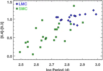
Figure4shows how the[6.4]−[9.3]color of the carbon stars depends on pulsation period. The larger sample considered here reinforces the previous conclusions. First, the DPR, as measured by the [6.4]−[9.3] color, generally increases with longer pulsation periods, once the period exceeds∼250days. Second, the scatter is signiﬁcant, with a range of DPRs possible at a given pulsation period. Third, the three galaxies considered show no obvious differences, indicating that metallicity does not have a noticeable effect.

Figure 1. Manchester method applied to the 5–15μm spectrum of MSXSMC159. The[6.4]−[9.3]color provides an estimate of the relative contributions of stellar photosphere and amorphous carbon dust in two spectral regions relatively free of absorption or emission features. Line segments are used to estimate the continuum under or over the C2H2 absorption band at 7.5μm, the Q branch of the C2H2band at 13.7μm, and the SiC dust emission feature at∼11.3μm.

(7)

4.2. Infrared Spectral Features

4.2.1. Silicon Carbide Dust

Figure 5 shows that the dependence of the strength of the SiC feature on the[6.4]−[9.3]color changes with host galaxy. For the Galactic sources, the SiC dust emission increases quickly from[6.4]−[9.3]=0 to∼0.4, then drops steadily to a color of ∼1.7, which is the maximum in the Galactic sample. Most of the carbon stars in the SMC sample behave differently, with SiC strength rising more gradually with color to [6.4]

−[9.3]∼1.4 for the reddest carbon star observed with the IRS in the SMC. The LMC sample is more evenly split between the upper and lower sequences.

Sloan et al. (2006) ﬁrst noticed this metallicity-dependent difference when they compared samples from the Galaxy and the SMC. As more carbon stars were added from the SMC (Lagadec et al.2007)and LMC(Zijlstra et al.2006; Leisenring et al. 2008), the two tracks in Figure 5 remained separate. Zijlstra et al.(2006)pointed out that metallicity will determine the availability of silicon, so that metal-rich stars generally populate the sequence with stronger SiC emission while metal-poor stars show weaker SiC features.

Table 5

Spectroscopic Data—IRS Sample

Target Eq. Width of FSiC/ [6.4]−[9.3] [16.5]−[21.5] FMgS/ IR Spectral

C2H2at 7.5μm Continuum (mag) (mag) Continuum Classiﬁcation

GM 780 0.162±0.010 0.316±0.006 0.403±0.008 0.165±0.024 K CE2

MSX SMC 091 0.146±0.015 0.147±0.007 0.528±0.007 0.073±0.025 K CE2 MSX SMC 062 0.117±0.006 0.062±0.003 0.675±0.008 0.174±0.024 K CE3 MSX SMC 054 0.177±0.006 0.179±0.003 0.756±0.004 0.101±0.016 0.191±0.021 CE3

2MASS J004326 0.196±0.007 0.080±0.006 0.234±0.019 K K CE1

MSX SMC 044 0.050±0.005 0.024±0.004 0.517±0.006 −0.101±0.046 K CE2 MSX SMC 105 0.184±0.008 0.157±0.005 0.866±0.003 0.226±0.022 0.254±0.029 CE3 MSX SMC 036 0.234±0.006 0.088±0.004 0.774±0.005 0.286±0.017 0.279±0.021 CE3 GB S06 0.113±0.005 0.058±0.002 0.969±0.003 0.284±0.020 0.358±0.025 CE4 MSX SMC 200 0.032±0.007 0.010±0.003 0.443±0.008 0.067±0.029 K CE2

Table 6

Spectroscopic Data—SWS Sample

Target Alias Eq. Width of FSiC/ [6.4]−[9.3] [16.5]−[21.5] FMgS/ IR Spectral

C2H2at 7.5μm Continuum (mag) (mag) Continuum Classiﬁcation

WZ Cas K 0.347±0.007 −0.022±0.002 0.029±0.002 0.438±0.004 K CE0 VX And K 0.238±0.001 0.182±0.001 0.123±0.003 0.067±0.010 K CE1 HV Cas K 0.090±0.001 0.226±0.001 0.353±0.002 −0.139±0.004 K CE2 R Scl K 0.290±0.002 0.205±0.001 0.273±0.002 0.266±0.002 0.292±0.004 CE1

R For K 0.125±0.001 0.279±0.001 0.361±0.001 0.131±0.003 K CE2

AFGL 341 V596 Per 0.063±0.001 0.073±0.001 1.665±0.005 0.407±0.008 0.411±0.010 CE5 CIT 5 V384 Per 0.065±0.001 0.305±0.002 0.682±0.001 0.323±0.002 0.186±0.002 CE3

U Cam K 0.078±0.001 0.327±0.001 0.107±0.002 0.157±0.004 K CE1

W Ori K 0.064±0.001 0.229±0.001 0.055±0.001 −0.054±0.004 0.137±0.002 CE1 IRC−10095 V1187 Ori 0.277±0.002 0.192±0.001 0.163±0.003 0.196±0.008 0.784±0.012 CE1

Figure 3.Distribution of the Galactic carbon stars in our control sample with [6.4]−[9.3] color, segregated by their infrared spectral classiﬁcations from Kraemer et al.(2002). The[6.4]−[9.3]color increases nearly monotonically along the sequence 1.NC–2.CE–3.CE–3.CR.

(8)

All eight of the stars with [6.4]−[9.3]2.0 have negative SiC/continuum ratios, which indicate SiC absorption in optically thick dust shells. The seven carbon-rich EROs observed by Gruendl et al. (2008) all show SiC absorption; two of these were re-observed as potential post-AGB objects by Matsuura et al. (2014). The eighth source was part of the SAGE-Spec program (Kemper et al.2010). All have spectro-scopic properties consistent with deeply embedded objects near the end of their AGB lifetimes.

4.2.2. Magnesium Sulﬁde Dust

Figure6shows how the MgS emission increases with [6.4]

−[9.3] in the different populations. MgS is apparent in the Galactic sample at all[6.4]−[9.3]colors, while in the LMC, the

ﬁrst MgS feature is at [6.4]−[9.3]∼0.25. No other LMC source shows MgS until [6.4]−[9.3] reaches a value∼0.5. In the SMC, MgS does not appear until[6.4]−[9.3]∼0.7.

Figure 7 illustrates the behavior of the MgS emission differently, by plotting the mean MgS/continuum strength for all data up to a given[6.4]−[9.3]color. It shows more clearly how the LMC lags the Milky Way, with the SMC even further behind, as the [6.4]−[9.3] color increases. The traces for the Milky Way and SMC are unchanged past colors of ∼1.6 and 1.4, respectively, due to a lack of redder sources. The lower abundances of Mg and S in more metal-poor stars appear to be delaying the condensation of MgS until the DPR is higher and the dust is cooler.

4.2.3. Acetylene Gas at7.5 mm

Figure 8 compares the behavior of the 7.5μm absorption band from C2H2for the different samples. For the less dusty stars ([6.4]−[9.3]0.35), all three galaxies show a range of band strengths, but to the red, the upper bound diminishes. Figure 9 clariﬁes the behavior of each galaxy by plotting the mean equivalent width and color for each CE class. For CE2 and redder sources, the mean equivalent width of the 7.5μm acetylene band is consistently strongest in the SMC and weakest in the Galaxy.

As shown below (Section 4.5), all of the CE0 and most of the CE1 sources are associated with relatively dust-free carbon

stars which can have strong molecular absorption bands due to the lack of veiling from the dust surrounding the redder sources. Sloan et al.(2015b)found that in the SMC, the dusty stars with veiled molecular bands usually are pulsating in the fundamental mode with strong amplitudes as Mira variables, while the other group are detected as semi-regulars or irregulars. To focus on the dust-production process, we should focus on the stars classiﬁed as CE2 or later.

Figure 5.Strength of SiC dust emission as a function of[6.4]−[9.3]color. As the[6.4]−[9.3]color increases, stars follow one of two tracks. The SiC strength increases quickly in more metal-rich stars, then turns over and decreases. In metal-poor stars, the SiC strength increases more gradually. Most of the stars with[6.4]−[9.3]2.0 have negative SiC strengths, indicating absorption.

Figure 6.Strength of MgS dust emission as a function of[6.4]−[9.3]color. More metal-poor stars have to have redder [6.4]−[9.3] colors before MgS becomes visible.

Figure 7.Cumulative mean MgS emission. At each color, the mean MgS/ continuum strength for all sources with bluer colors is plotted.

(9)

To make a quantitative comparison of the 7.5μm acetylene band, we examine the CE2–3 sources, because the CE4 and CE5 classes have only one SMC source each. We set negative equivalent widths to zero, because 7.5μm emission is unlikely. For the chosen color range, the mean equivalent width of the 7.5μm band decreases from 0.12±0.01μm in the SMC to 0.10±0.01μm in the LMC and to 0.08±0.02μm in the Galaxy (the quoted errors are the uncertainty in the mean). While the spread in each sample is substantial, the steady drop in mean band strength is still apparent. Thus the expanded IRS sample has not changed the conclusions drawn before about the 7.5μm acetylene band.

While the behaviors of the C2H2absorption at 7.5μm and the SiC emission at 11.5μm differ quantitatively, their rough similarity raises a possible concern, which we have examined and ruled out. Acetylene also shows a strong absorption band centered at 13.7μm, but the sharp absorption band apparent at 13.7μm is just from the Q branch(ΔJ=0), with the P and R branches extending the feature over a micron in either direction. The possible SiC emission could be affected by strong C2H2 absorption to the red, which could push the continuum fit down and artifically add to the measured emission. We investigated by shifting the wavelengths used tofit the continuum on the red side of the SiC feature. Figure1

shows an inflection on the SiC feature at∼12.0μm. We shifted the red continuum wavelengths to this inflection and recalculated the intregated SiCflux for our samples, and found that, while the total SiC emission certainly grew smaller, the samples behaved the same qualitatively, and the differences in how the three galaxies behaved were unchanged.

4.3. Bolometric Magnitudes

For each star in the Magellanic sample, we can estimate its bolometric magnitude (Mbol)by integrating its SED, which is determined from the IRS spectra and the mean magnitudes from the multi-epoch photometry described in Section2.4. We integrated through the photometry below 5μm using linear interpolation, then integrated the IRS spectrum. To the blue of the optical photometry, we assumed a Wien distribution. To the red of the IRS data, we assumed a Rayleigh–Jeans tail. If the IRS spectrum only included data from SL (i.e., stopped at

14μm), we also utilized the MIPS data at 24μm. The resulting estimates forMbolappear in the last column of Table4.

Our IRS sample includes six carbon stars in NGC419. At an assumed distance modulus of 18.90, the median absolute magnitude for these stars=−4.79±0.23, with Mbol=−5.24 for NGC419 IR1 and −4.73 for NGC419 MIR1. These values are consistent with an estimated zero-age main-sequence mass of 1.9M_e(Kamath et al. 2010)and an age of 1.35 Gyr (Girardi et al. 2009), based on models of the AGB and red clump, respectively. The bolometric magnitudes of NGC419 compare well with the rest of the SMC, which has

áMbolñ = -5.030.49. If NGC419 were in front of the

SMC at a distance modulus of 18.50(Glatt et al.2008), then its median Mbol would lie outside the 1σ range for the SMC, making it older than most of the carbon stars observed by the IRS in the SMC.

Figure 10 includes evolutionary tracks from Vassiliadis & Wood (1993)on the period–luminosity plane and also shows the location of the P–L relation for fundamental-mode pulsators. For stars with higher initial mass and for lower-mass stars with longer periods, the evolutionary tracks are nearly horizontal, so thatMbolcan be used as a proxy for initial mass. We have therefore divided the fundamental-mode pulsators into four mass bins with the horizontal lines deﬁned in Figure10 as boundaries. While the evolutionary tracks do deviate from horizontal for shorter pulsation periods, theﬁgure shows that this has little impact on the stars in our sample, provided we only consider stars with periods 250 days (logP∼2.4).

It should be emphasized that the estimates for initial mass are rough and are not to be taken too literally or quantitatively. The key is the steady bolometric magnitude on the late stages of the evolutionary tracks. These make it possible to use Mbol to segregate the data by initial mass for statistical purposes.

The thick black dashed line in Figure 10 is a period– luminosity relation,firstfitted to all of the Magellanic stars in our sample with periods >250 days, then fitted iteratively to only those within an envelope of±0.9 mag to avoid stars not on the fundamental-mode sequence. The linear solution Figure 9.Strength of the 7.5μm C2H2absorption band vs.[6.4]−[9.3]color,

binned by CE class to illustrate the general trends in the data. When determining means, negative equivalent widths have been treated as zero, because acetylene emission is unlikely.

(10)

converges quickly:

( ) ( )

=

-Mbol 2.30 2.74 logP days . 1

This line is steeper than the P–L relation by Whitelock et al. (2006). They found a slope of −2.54 using bolometric corrections to estimate Mbol, while our estimates are based on integrations through the IRS data and the available photometry at shorter wavelengths. Sloan et al. (2015b) noted that the estimated bolometric magnitudes of the dustiest sources, which tend to have the longest periods, depend on the precise method used. Here, we have spectral data covering the peak of the SED for those sources, which should improve on the cases where only photometry is available.

4.4. The Period–Color Relation and Initial Mass

Figure11reprises Figure4, except that the sources are color-coded by our rough estimates of their initial mass. Figure 11

explains the width of the relationship of [6.4]−[9.3] versus period. The Magellanic samples include a range of masses, each of which follows its own narrow relation. When stars switch from overtone pulsations to the fundamental mode, they begin to produce dust at significant rates for thefirst time, and this rate increases as their pulsation period increases. The slope to the period–luminosity relation means that this mode switch occurs at longer pulsation periods for more luminous(and thus more massive)stars, which explains why segregating by mass reveals the parallel tracks in Figure11. The finite width of the period–luminosity relation suggests that this scenario of increasing pulsation period and increasing DPR and mass-loss rate can be sustained for a limited time.

Sloan et al. (2008) concluded that for Magellanic carbon stars, metallicity did not play a detectable role in dust production, because the Galaxy, LMC, and SMC showed indistinguishable relations between [6.4]−[9.3] color and pulsation period. However, more metal-poor carbon stars in other nearby Local Group dwarf galaxies ([Fe/H]−1) do

show less dust than might be expected for their pulsation period (Sloan et al.2012).

The data in Figure11 point to the need to account for the different mass distributions of the carbon stars observed by the IRS in the LMC and SMC in order to re-assess if the role of metallicity can be detected for[Fe/H]−1. A lineﬁtted to all of the data gives

[6.4]–[9.3] = -4.52+1.91 logP(days .) ( )2

For each star, we used this line to predict the expected [6.4]

−[9.3]color based on the pulsation period and compared it to the observed[6.4]−[9.3]color. For each mass bin and for each galaxy, we computed the median of these offsets. Table7gives the difference in these median offsets, along with the propagated uncertainty in the mean (in the column labeled

“Using One Fitted Line”). Averaging the differences between LMC and SMC across the mass bins reveals a redder [6.4]

−[9.3]color in the LMC of 0.125±0.042 mag, which is a 2.9σ result.

The data in each mass bin in Figure11follow a steeper slope than the total data set, and the carbon stars in the LMC and SMC do not have the same period distributions. To further correct for this difference in the sample, we haveﬁtted lines independently to the four mass bins. Because these lines are driven somewhat by the noise in our data, we found the weighted mean of the slopes (2.91 mag/dex) and used this slope for each mass bin. The colored dotted lines in theﬁgure illustrate the results. Table 7 gives the resulting median difference in [6.4]−[9.3] between the LMC and SMC. The average from the four mass bins is 0.054±0.040, which is only a 1.3σ result.

We conclude that the full sample of Magellanic carbon stars observed by the IRS shows hints of a subtle dependence of DPR with metallicity, but once we account for different distributions by initial mass and metallicity, our sample does not reveal a statistically signiﬁcant result. The effects of pulsation period and initial mass on dust production are much stronger.

4.5. Color–Color and Color–Magnitude Space

Carbon stars fall along a well-deﬁned sequence in most infrared color–color diagrams, with each color increasing steadily and monotonically as the DPR increases. The [5.8]

−[8]color is an exception, because it is sensitive to both dust content and the strength of molecular absorption in the 5.8μm

ﬁlter (Srinivasan et al. 2011). Figure 12 plots the [5.8]−[8] color versusJ−Kin the top panel. From J−K∼1.3 to 2, increasing molecular absorption reddens [5.8]−[8], but for Figure 11. [6.4]−[9.3] color as a function of pulsation period with the

Magellanic sample, color-coded by their initial mass as estimated from their bolometric magnitude. Sources not assigned to a mass bin are not included. The width of the relation between[6.4]−[9.3]color and period clearly arises from the mass distribution of the samples. The gray dashed line is a lineﬁtted to all of the data, while the colored dotted lines areﬁtted to each mass bin separately

(see Section4.3).

Table 7

Period-corrected Differences in[6.4]−[9.3]Color

Approximate Δ(LMC)–Δ(SMC) (mag)

a

Initial Mass(Me) Using One Fitted Line Fitting to Each Mass Bin ∼4 0.083±0.098 −0.001±0.077

∼3 0.147±0.100 0.054±0.103

∼2 0.112±0.048 0.032±0.043

∼1 0.157±0.093 0.131±0.100

Note.

a_Δ₌

(11)

J−K2, increasing dust opacity is the culprit. Sloan et al. (2015b)called these two sequences“molecular”and“dusty”to identify the agent responsible for the reddening. They found that semi-regular variables dominate the molecular sequence (J−K2), while Mira variables dominate the dusty sequence. This difference is not between overtone and fundamental-mode pulsators, as half of the semi-regulars are pulsating in the fundamental mode. Rather, it is a difference between stars pulsating with small and large amplitudes. Generally, it is the latter that are associated with dust production.

The bottom panel of Figure12presents the sample in a more familiar near-IR CMD. Blum et al.(2006)labeled the sequence extending to the red of J−Ks∼2 as the “extreme” AGB stars,18but this terminology is something of a misnomer, as the objects are only extreme in the sense that they are producing carbon-rich dust, something that all carbon stars must do before they end their lives on the AGB. Superlatives like “extreme” are more appropriate for the EROs discovered in the LMC by Gruendl et al. (2008). These are the deeply embedded carbon stars analogous to targets in the Galaxy like AFGL 3068(e.g., Jones et al.1977; Lebofsky & Rieke1977). We will follow the practice of Sloan et al. (2015b) and refer to objects with

J−Ks2 as“dusty”carbon stars, by which we mean carbon stars associated with signiﬁcant and readily measurable quantities of dust.

Figure13replaces theJandKsﬁlters in Figure12with[3.6] and [4.5]. In all four panels of the two plots, the [6.4]−[9.3] color generally increases along the sequence from blue to red, but with some scatter. This scatter appears in any color chosen, and it is consistent with what one would expect from variations in DPR as a function of time, with bluer colors sensitive to warmer and more recently formed dust.

The CE1 sources (0.05<[6.4]−[9.3]<0.35) straddle the boundary between the molecular and dusty sequences in both

ﬁgures. On the molecular sequence, the overlap between CE0 and CE1 is complete, despite the presence of more dust in the CE1 sources, and it shows that the dust is not determining position on this sequence. The vertical spread of the molecular sequence in the bottom panel of Figure13shows that the[3.6]

−[4.5]color is less sensitive to molecular bands thanJ−Ks. In Figure 12, none of the CE5 stars ([6.4]−[9.3]>1.25) follow the relationship between [5.8]−[8] and J−Ks estab-lished by the sources with less dust. If they did, they would be off the right-hand edge of the plot, provided we could detect them atJand Ks. Because these sources are so embedded, if they followed the dusty sequence, they would actually be below the detection limit of the near-IR surveys we examined. Of the 21 CE5 sources, we have validJ−Kscolors for only nine, and all appear with bluer J−Ks colors than the dusty sequence would lead us to expect. In the bottom panel, all of the CE5 sources plotted are also off the sequence. Their behavior is fully consistent with a shift to bluerJ−Kscolors. Several of the CE4 and even some CE3 sources can also be seen to have shifted. In Figure13, no sources are missing, and Figure 12. Color–color and color–magnitude diagrams featuring theJ−Ks

colors on the horizontal axis. Symbols are coded for galaxy with shape and for [6.4]−[9.3] color with color. The [6.4]−[9.3] intervals correspond to the CE0–5 classiﬁcations. None of the CE5s and only about half of the CE4s follow the sequences. (CE4: 0.95<[6.4]−[9.3]<1.25; CE5: [6.4] −[9.3]>1.25.)

Figure 13.Color–color and color–magnitude diagrams featuring the [3.6]– [4.5]colors on the horizontal axis. Symbols are coded for galaxy with shape and for[6.4]−[9.3]color with color. The[6.4]−[9.3]intervals correspond to the CE0–5 classiﬁcations. Only a handful of the reddest sources in[5.8]−[8] are off the sequence, along with one CE4.

18

(12)

the number of off-sequence sources is greatly reduced, with only a few CE5 sources not on the dusty sequence in either panel.

As noted in Section2.4, it is only for the deeply embedded sources that a photometric mismatch is a danger, and even then the odds of a mismatch are slight for a given source. We conclude that most or all of our off-sequence sources have colors indicative of the source itself and not a chance superposition of two sources in the search beam.

4.6. Variability

If the off-sequence sources in Figure 13have really moved off the AGB, then the amplitude of their variability should have dropped. Figure14plots the variability amplitude of all of our carbon stars as a function of[5.8]−[8]color. The values plotted are the standard deviations (σ) of the mean magnitudes in Tables 3 and 4. For a pulsation cycle which follows a sine function, the peak-to-peak amplitude=2 2s.

As the stars shift from CE0 (nearly naked) to CE5 (very dusty), the amplitude of their variability increases as they grow redder, but once [5.8]−[8] reaches a value of ∼1.5, the amplitude begins to decline. The three sources furthest from the carbon sequence in the top panel of Figure 13 are all in GroupA in the bottom right-hand corner of Figure 14. These are both the reddest and the least variable sources in the sample. More recent photometry of the reddest carbon stars in the LMC at 3.6 and 4.5μm extends the temporal baseline and conﬁrms the trend of decreasing variability with increasing [5.8]−[8]color (B. A. Sargent et al. 2016, in preparation).

Had we chosen to use the variability amplitude at 3.6μm instead of 4.5μm, the results would have been the same qualitatively. Dropping the color corrections derived in Appendix A also does not change the result qualitatively. It does change the apparent variabilities quantitatively, increasing the apparent amplitudes for the stars which are most variable because it increases the apparent scatter in the data, but for the relatively non-variable sources, this effect is much smaller. By using the 4.5μm data, we have reduced possible errors from the corrections even more, since theWISE-to-IRAC corrections are much smaller at 4.5μm than at 3.6μm.

Four more sources appear to be relatively non-variable for their [5.8]−[8]color, and are labelled as Groups B and C in Figure14. Group C includes one CE4 source (red diamond), SAGE J054546, which is also off-sequence in the bottom panel of Figure13. The remaining three are all CE5, and except for unusually low-variability amplitude, none stands out in any other signiﬁcant way.

5. DISCUSSION

5.1. Evolution off the AGB

The three sources most clearly off the carbon sequence in the color–color diagram in Figure 13 have [5.8]−[8]>2.5 and [3.6]−[4.5]<3. They are IRAS05133, IRAS05191, and IRAS05260, in order of increasing [3.6]−[4.5] color. The other two sources with [5.8]−[8]>2.5 are IRAS05026 and IRAS05042. Group A in Figure14consists of theseﬁve stars. They are much less variable than the rest of the sources with [5.8]−[8]1.5. And all ﬁve are also SiC absorption (CA) sources.

In the top panel of Figure 12, the only CA source with a

J−Ks color is IRAS05133, and it is bluer than any other carbon star in our sample! Whatever has led to its unusually blue[3.6]−[4.5]color has allowed us to detect an even bluer source atJandKs. WithKs=16.6 andJ=17.4, it is just at the detection limit. The other four sources are redder at [3.6]

−[4.5], have more extinction in the near-IR, and consequently are undetected atJandKs.

Thus theﬁve most embedded carbon stars in our sample(as measured with [5.8]−[8]) have properties consistent with evolution off the AGB. Their variability is lower than the less embedded sources, they show SiC absorption, indicating high column densities of dust, and three appear to be developing double-peaked SEDs as the central star becomes visible.

However, other stars are relatively non-variable, and others also show SiC absorption. Of the other non-variable sources, all but SAGE J054546(CE4)are either CE5 or CA5(i.e.,[6.4]

−[9.3]>1.25). These sources may be approaching the end of their AGB evolution.

The steady decline in variability past [5.8]−[8]∼1.5 (Figure14)suggests that more than just the handful of sources most obviously off of the sequences in Figure 13 are approaching the end of their AGB lifetimes.

5.2. Non-spherical Dust Shells

For the off-sequence sources, the excess blueﬂux indicates that we are able to peer into the dust and glimpse the central star, either directly or through scattered light. The dust envelope may be growing patchy or it may be distributed asymmetrically, perhaps in a torus or possibly even a disk.

Figure 12 reveals other sources which do not follow the carbon-star sequence atJandKs, even though they are on the sequence in the longer-wavelength ﬁlters in Figure 13. In particular, a number of CE4 sources(in red)are off-sequence in both panels of Figure12, with much bluerJ−Kscolors than expected for either their [5.8]−[8] colors or Ks magnitudes. More of the CE5 sources also behave similarly.

The opacity of amorphous carbon dust drops as∼λ−2, making it difﬁcult to explain how we could directly observe the central source atJandKbut not at 3.6 and 4.5μm. If we are detecting the central source via light scattered above and below a disk or in the polar regions of an asymmetric dust shell, then Figure 14.Amplitude of the variability at 4.5μm(as measured by the standard

(13)

we would expect to see a bluer color at J−Ks than at [3.6]

−[4.5], because the scattering efﬁciency drops asλ−4. Bernard-Salas et al.(2006)proposed scattering in a system with a disk viewed close to edge-on to explain the unusual object SMPLMC011, which presents an optically thick carbon-rich dust spectrum with molecular absorption bands in the infrared but shows Hαin emission in the optical. Sloan & Egan(1995)

suggested scattering from the poles of an asymmetric dust distribution in the embedded Galactic carbon star IRC+10216 to explain emission from relatively warm dust above and below the central source. This hypothesis could be tested for the embedded Magellanic carbon stars by measuring their polarization as a function of wavelength in the near-IR.

The nature of the dust geometry has significant conse-quences. Sloan & Egan (1995) noted that the deviation from spherical symmetry they argued for in IRC+10216 was subtle and did not prevent spherically symmetric radiative transfer models from working. Disks are a different story. Their non-isotropic emission would lead to significant uncertainties in bolometric luminosities and thus our basic knowledge about the sources. Boyer et al.(2012)noted that the ten dustiest AGB stars detected in the SAGE surveys of the SMC accounted for 17% of the total dust input to the galaxy when assuming spherical symmetry. If the dust in embedded carbon stars were in disks and not outflowing shells, the amount of dust produced by AGB stars would have to be revised downward, because the DPR scales with outflow velocity, which in disks would be zero.

Disks imply binarity, which leads to more consequences. Equatorial disks can result from binaries interacting during the AGB phase(e.g., Soker & Livio1989). If the sources we have identified as off-sequence are interacting binaries, then they may have have never been on sequence and are instead following a different evolutionary path in color–color space. High-resolution imaging of Galactic sources show that binary interactions are not rare at all. The Mira variable R Scl is embedded in a spiral structure indicative of interactions of the outflows from the carbon star with a companion (Maercker et al. 2012). L2 Pup, the nearest AGB star in the sky, has a dusty disk, evidence of a companion, and the beginnings of bipolar nebulosity (Kervella et al. 2014, 2015). These observations add to the evidence that binaries and their interactions on the AGB strongly influence the structure of post-AGB objects and planetary nebulae(PNe) (e.g., Lagadec & Chesneau 2014; Jones2015).

As already stated, near-IR polarimetry of the most embedded carbon stars in the present sample would help diagnose the geometry of these systems. Radiative transfer modeling would also help by translating the constraints imposed by the SEDs to constraints on the dust morphology.

5.3. SiC and Luminosity

Carbon stars in the SMC generally show very little SiC emission compared to their counterparts in the LMC and the Galaxy, but there are exceptions. Sloan et al.(2006)foundﬁve stars in the SMC that had signiﬁcantly more SiC for their[6.4]

−[9.3] color, and the present sample adds two more SiC-rich sources, both with bluer [6.4]−[9.3]colors than the otherfive (see Figure 5). Sloan et al. (2006) examined a number of properties for thefive SiC-rich stars in their sample and could not find anything that distinguished them besides their SiC emission strength.

To compare the SiC-rich and SiC-poor sources in the current sample, we concentrate on[6.4]−[9.3]colors between 0.35 and 0.95 (CE2–3), where the two tracks are most distinct, and consider the sources above and below SiC/continuum=0.125 separately. In the SMC, the mean bolometric magnitude for the SiC-rich group is −5.05±0.41, compared to −5.08±0.50 for the SiC-weak group. The uncertainties in the mean are 0.17 and 0.11, respectively. The two groups are indistinguishable in luminosity, which implies that they have similar mass, age, and metallicity distributions.

In the LMC, the SiC-rich group has Mbol=−4.91±0.45, versus−5.20±0.53 for the SiC-poor group. The uncertainties in the mean are 0.08 and 0.09, respectively. While the separation is larger and more statistically signiﬁcant, it is in the opposite sense to what we might expect, with the more luminous stars, which presumably would be more massive and more metal-rich, associated with the weaker SiC features.

Thus, while the relative numbers of stars showing strong and weak SiC emission in the Galaxy, LMC, and SMC support the hypothesis that the strength of the SiC feature is tracing metallicity, we ﬁnd no support for the hypothesis within a given galaxy. Sloan et al.(2006)were unable to explain why some sources in the SMC showed strong SiC emission while most did not, and we are unable to improve on that situation.

5.4. Layered Grains

Lagadec et al. (2007) suggested that the condensation sequence of SiC and amorphous carbon differed in metal-rich and metal-poor stars, with SiC formingfirst in the Galaxy and later in the SMC. Leisenring et al. (2008) followed with a proposal for multiple evolutionary tracks for dust grains, with the extremes determined by whether SiC or amorphous carbon formed first. Figure 15 simplifies the proposal of Leisenring et al. (2008) and presents two tracks consistent with the infrared properties of Galactic and Magellanic carbon stars. The key is that the dust grains must be layered, which may Figure 15.Possible scenario for the evolution of dust grains, modeled on a

(14)

wreak havoc with attempts to use the grain properties to estimate the masses of the refractory elements in dust grains.

MgS is a case in point. MgS grains do not form until the dust shells pass an optical thickness limit which depends on the metallicity of the sample, as Figures6 and 7show. The MgS could condense as grains independently, but then, in order to explain the strength of the MgS feature in post-AGB objects and young PNe, more S would be required than can exist around these stars. On these grounds, Zhang et al. (2009)

argued that MgS could not be the carrier of the 26–30μm feature.

Zijlstra et al.(2006)proposed that MgS formed as a layer on pre-existing seeds of SiC and amorphous carbon. Lombaert et al.(2012)argued that the optical properties of a grain coated with MgS would mimic those of a solid MgS grain, which would account for the strength of the MgS feature in PNe without violating abundance constraints. Sloan et al. (2014)

explained why other concerns raised about MgS as the carrier of the 26–30μm feature can be discarded. All of the evidence is consistent with MgS forming a layer on carbonaceous grains, with the condensation trigger depending on metallicity.

However, it is unlikely that any of the layers are pure. The metal-rich track suggests that metal-rich carbonaceous grains should consist of SiC cores surrounded by amorphous carbon mantles. In the most optically thick dust shells, these would be mostly coated by MgS, and yet the spectra from these sources show absorption from SiC. Thus some SiC must be present within one optical depth of the surface of the grains, which means that not all grains are coated with MgS, or the coatings are incomplete. Furthermore, if the grains consist of a SiC core and an amorphous carbon mantle, that mantle cannot be pure and must also contain some SiC.

Young carbon-rich PNe in the LMC and SMC often show unusually strong emission features at∼11.5μm in their spectra (Bernard-Salas et al.2009). Sloan et al.(2014)showed that the shape of these features was consistent with SiC dust, modiﬁed by the presence of emission from polycyclic aromatic hydrocarbons. From abundance arguments, one would expect weaker SiC emission in more metal-poor objects, but the opposite is true, with carbon-rich Magellanic PNe showing stronger SiC emission than in the Galaxy. Sloan et al.(2014)

suggested that photoprocessing of carbonaceous grains would preferrentially remove amorphous carbon from the surface, resulting in grains coated by SiC. Such a scenario would require some intermixing of SiC and amorphous carbon in the outer layers of the grains.

The available observational evidence points to layered grains with a structure more complicated than depicted in Figure15. The strength of the SiC and MgS features with increasing[6.4]

−[9.3]color points to two tracks as shown, but the presence of SiC absorption in the most embedded sources and the strength of the SiC feature in young PNe requires some SiC in the layers of the grains within one optical depth of the surface.

5.5. Completeness

The pointed nature of spectroscopic samples introduces biases, which can make it challenging to compare different populations. This work has focused on using properties like the pulsation period of the star or the[6.4]−[9.3]color, which is a proxy for the amount of dust, as the independent variable in order to compare sources with similar properties when examining other properties such as the strength of emission

features from SiC or MgS dust. A key result is that the amount of dust produced by a star in the Galaxy, LMC, or SMC, depends primarily on its pulsation period and initial mass. The effect of metallicity is unclear with the current sample. While we do see hints of less dust in more metal-poor stars when controlling for period and mass, this decrease is not statistically signiﬁcant in the IRS samples.

In contrast, van Loon et al.(2008)found a clearer difference in the dust content of their sample of carbon stars in the SMC, compared to a similar study in the LMC(van Loon et al.2006). They drew this conclusion from a spectroscopic study of the absorption bands from C2H2 at 3.1 and 3.8μm, ﬁnding that dust veiling affected the bands more in the LMC than in the SMC. Figure 16 plots the [6.4]−[9.3] color for the stars in common between their sample and ours as a function of pulsation period and shows that while the carbon stars in the LMC have more dust on average than their counterparts in the SMC, the two samples have different distributions in pulsation period, as well. None of the carbon stars in the LMC in common with the IRS sample have a period less than 500 days, compared to over half the SMC sample. Given the differences in the LMC and SMC samples, one would expect the stars in the LMC to show more dust, simply because they are pulsating with longer periods.

The IRS-based studies have concentrated on comparing like with like, which means comparing the dust content in stars with similar pulsation periods. Previous studies with the IRS on

Spitzer have found little dependence of the dust content on metallicity in carbon stars. The larger sample considered here has not changed that result.

However, the evidence is building that the populations of carbon stars in LMC and SMC differ. Figure16shows that the 3μm samples contain more longer-period pulsators and dustier carbon stars in the LMC than the SMC. The IRS samples show a similar difference in the two galaxies. In the SMC sample, the reddest[6.4]−[9.3]color is 1.4, so that only one SMC source out of 40, NGC419 MIR1, is classiﬁed as CE5, compared to 20 CE5 and CA5 sources out of 144 in the LMC, 15 of which are redder than NGC419 MIR1, with [6.4]−[9.3] colors extending past 3.0. At ﬁrst glance, this could easily be a selection effect, as is often the case for spectroscopic samples, Figure 16.Samples of Magellanic carbon stars studied by van Loon et al.