Scholarship@Western
Scholarship@Western
Electronic Thesis and Dissertation Repository
8-15-2018 10:30 AM
Computing, Modelling, and Scientific Practice: Foundational
Computing, Modelling, and Scientific Practice: Foundational
Analyses and Limitations
Analyses and Limitations
Filippos A. Papagiannopoulos The University of Western Ontario
Supervisor Myrvold, Wayne
The University of Western Ontario Graduate Program in Philosophy
A thesis submitted in partial fulfillment of the requirements for the degree in Doctor of Philosophy
© Filippos A. Papagiannopoulos 2018
Follow this and additional works at: https://ir.lib.uwo.ca/etd
Part of the Logic and Foundations of Mathematics Commons, and the Philosophy of Science Commons
Recommended Citation Recommended Citation
Papagiannopoulos, Filippos A., "Computing, Modelling, and Scientific Practice: Foundational Analyses and Limitations" (2018). Electronic Thesis and Dissertation Repository. 5660.
https://ir.lib.uwo.ca/etd/5660
This Dissertation/Thesis is brought to you for free and open access by Scholarship@Western. It has been accepted for inclusion in Electronic Thesis and Dissertation Repository by an authorized administrator of
This dissertation examines aspects of the interplay between computing and scientific practice.
The appropriate foundational framework for such an endeavour is rather real computability
than the classical computability theory. This is so because physical sciences, engineering, and
applied mathematics mostly employ functions defined in continuous domains. But, contrary
to the case of computation over natural numbers, there is no universally accepted framework
for real computation; rather, there are two incompatible approaches –computable analysis and BSS model–, both claiming to formalise algorithmic computation and to offer foundations for scientific computing.
The dissertation consists of three parts. In the first part, we examine what notion of
‘algorithmic computation’ underlies each approach and how it is respectively formalised. It is
argued that the very existence of the two rival frameworks indicates that ‘algorithm’ is not one
unique concept in mathematics, but it is used in more than one way. We test this hypothesis
for consistency with mathematical practice as well as with key foundational works that aim to
define the term. As a result, new connections between certain subfields of mathematics and
computer science are drawn, and a distinction between ‘algorithms’ and ‘effective procedures’ is proposed.
In the second part, we focus on the second goal of the two rival approaches to real
computa-tion; namely, to provide foundations for scientific computing. We examine both frameworks
in detail, what idealisations they employ, and how they relate to floating-point arithmetic
sys-tems used in real computers. We explore limitations and advantages of both frameworks, and
answer questions about which one is preferable for computational modelling and which one for
addressing general computability issues.
In the third part, analog computing and its relation to analogue (physical) modelling in
science are investigated. Based on some paradigmatic cases of the former, a certain view about
the nature of computation is defended, and the indispensable role of representation in it is emphasized and accounted for. We also propose a novel account of the distinction between
analog and digital computation and, based on it, we compare analog computational modelling
to physical modelling. It is concluded that the two practices, despite their apparent similarities,
are orthogonal.
Keywords: Definitions of Algorithms, Real Computability, Computable Analysis, Type-2 Turing Machines, BSS Model, Real-RAM, Foundations of Scientific Computing, Epistemology
of Simulations, Conceptual Analysis, Idealisations, Formalisation of Mathematical Concepts,
Decidability in Physics, Analog Computation, Physical Models, Analog and Digital, Philosophy
of Computing, Representation, Open Texture
I would like to express my deep gratitude to my supervisor, Professor Wayne Myrvold, for
his incisive comments and criticisms during the long process of writing this dissertation, as well as for all his advice and support. He has been particularly influential on my philosophical
development and thinking. This dissertation would have been very different (indeed, even in a different area), had I not met him. For all of my intellectual debt, I would like to offer my deepest thanks.
I would like to express my very great appreciation to Professor Robert DiSalle, for the
tremendously inspiring discussions, since my very first year in the program, the long support,
the generosity, and the kindness. For all that, I’m profoundly grateful. I am also deeply indebted
to Professor John Bell for being a great inspiration to me, through our unforgettable, stimulating
discussions. I would also like to offer my special thanks to the Rotman Institute of Philosophy, for the stimulating environment and the workspace, and for all the material support.
Special gratitude is owned to Michael Cuffaro. His continuous support, confidence, help, and feedback on parts of the content of this dissertation had a hugely beneficial effect on my graduate school experience. I hope that I will continue to be honoured by his friendship and
kindness for years to come.
Finally, although neither directly nor indirectly involved with this project, Professor Stathis
Psillos has made a huge impact on my thinking, being a teacher, mentor, and friend, since I
decided to undertake the Master’s program in History and Philosophy of Science at the University
of Athens. I’m very grateful for everything during these last eight years, and especially for instilling in me the desire to produce the best work I’m capable of.
and to my brother.
Abstract i
Acknowlegements ii
List of Figures 1
1 Introduction 2
1.1 The Church-Turing thesis: some background . . . 3
1.2 Is the Church-Turing thesis inadequate for real functions? . . . 5
1.3 Two very different approaches . . . 6
1.3.1 The BSS model . . . 6
1.3.2 Effective Approximation . . . 7
1.3.3 Incompatibility between the two main approaches . . . 11
2 Algorithms 15 2.1 The BSS/Real-RAM in other areas of mathematics . . . 17
2.2 The problem about algorithms . . . 19
2.2.1 Three levels of formalisation . . . 20
2.2.2 Three possible interpretations . . . 21
2.2.3 Algorithm: the informal concept . . . 23
2.2.4 The problem reformulated . . . 24
2.3 Historical context . . . 25
2.4 Theoretical context . . . 31
2.4.1 Turing . . . 32
2.4.2 Kolmogorov and Uspensky . . . 32
2.4.3 Turing’s and K&U’s conceptualisations . . . 34
2.4.4 The idealisations strike back: Moschovakis and Gurevich . . . 36
2.5 What the historical and theoretical investigations tell us . . . 40
2.6 Which of the three interpretations? . . . 42
2.7 Conclusions . . . 46
3.1 Scientific computing . . . 51
3.2 Intuitions . . . 52
3.3 Why the BSS/Real-RAM models work . . . 54
3.3.1 Idealisations in scientific representation and the principle of regularity . 55 3.3.2 BSS/Real-RAM as idealised representations . . . 56
3.3.3 When the idealisations fail . . . 60
3.4 Which foundations? . . . 61
3.5 Conclusions . . . 62
4 Computing and Modelling: Analog vs. Analogue 63 4.1 Historical examples of mechanical computing devices . . . 64
4.2 Differential Analysers and the General Purpose Analog Computer . . . 69
4.3 Accounts of ‘Analog’ . . . 74
4.3.1 Accounts based on intrinsic properties of the computational machines. . 75
4.3.2 Accounts based on representational properties. . . 77
4.4 A comment on the nature of computing . . . 79
4.5 Against the analogy view of ‘analog’ . . . 84
4.6 Continuous vs. discrete representations . . . 86
4.6.1 Goodman’s account . . . 88
4.7 Analog vs. digital computation: the proposed account and concluding remarks . 90 4.8 Physical models . . . 96
4.8.1 Kinds of physical models . . . 96
4.8.2 Working example: flow around an aeroplane wing . . . 97
4.9 Comparison with analog computing . . . 100
4.10 Summary and directions for further research . . . 103
5 Summary and Conclusions 105
Bibliography 109
1.1 BSS implementation of Newton’s method . . . 7
1.2 Floor and step functions . . . 13
1.3 Two articles in theNotices of AMSoffering foundations for scientific computing 14 2.1 Margarita Philosophica(1503, woodcut) . . . 26
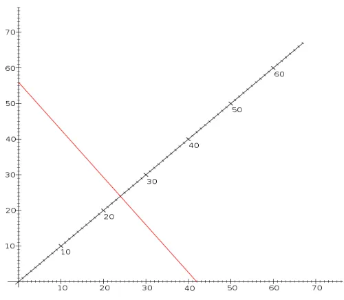
4.1 A nomogram for computing a two-variable functionT(S,R) . . . 65
4.2 A nomogram for computing 1z = 1x + 1y . . . 65
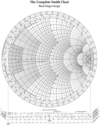
4.3 A Smith Chart . . . 66
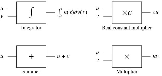
4.4 Operations performed by GPAC units . . . 69
4.5 A circuit for solving ¨y=−y . . . 71
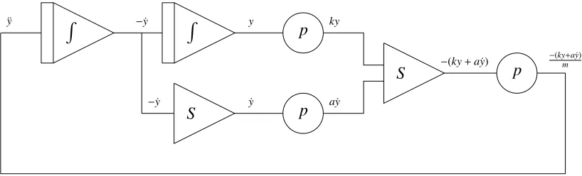
4.6 Analog computing diagram for the damped spring-mass system. . . 73
4.7 An integrator circuit . . . 74
4.8 An electronic circuit implementing the analog computer for damped spring-mass system . . . 74
4.9 Addition with concentric discs. . . 85
4.10 Multiplication with cogwheels or discs in contact . . . 86
4.11 Computation involves two kinds of representation . . . 91
4.12 Babbage’s Differential Engine (detail) . . . 94
4.13 Scale model and prototype of an airfoil. . . 99
4.14 Simulation of airflow around a wing on an analog electronic computer. . . 102
Chapter 1
Introduction
Most of us become familiar with algorithmic routines from our very early school years. We are taught how to perform operations, such as multiplication and long division, in a rather
mechanical manner. Constructing truth-tables, finding least common multiples, or solving
systems of linear equations by Gaussian elimination are also some examples of such mechanical
thinking, still at a high-school level.
So the notion of ‘algorithm’, although informal, has for the most part been taken as
unprob-lematic among mathematicians, and of no need for further formalisation. And when the need to
make it more rigorous arose,1 all offered mathematical models of algorithmically computable functions over the integers were actually proved equivalent; a fact that justified the certainty that
thereis oneclear underlying concept of ‘algorithmic computation’. Nevertheless, the situation turned out to be different when mathematicians tried to do the same for algorithmic computation of real-valued functions. Two very different traditions of computation have emerged, within which the notion of ‘algorithm’ is formalised in different, and often incompatible, ways. Both traditions have for the most part run a parallel non-intersecting course. Both are motivated by
a desire to understand the essence of computation and of algorithm. Both aspire to discover
useful, even profound, consequences (Blum, 2012), and both claim to offer a foundation for scientific computing (Blum 2004, Braverman and Cook 2006).
A basic aim of this work is to draw attention to these conceptual problems from the point of
view of philosophers of (science and) mathematics, interested in the foundations of (scientific)
computation. The strikingly limited philosophical literature on real computability is focused on arguing for one or the other of the rival models. But, to the author’s knowledge, the implications
of this situation for our conceptual understanding of ‘algorithm’ has gone unnoticed. A second
aim is to connect important works on algorithms and computation that have mainly existed in
parallel. Thus, I draw upon certainconceptual analysesof ‘algorithms’, coming from computer
1More details about this are in the next section.
science and logic, to account for the apparently incompatible pictures of ‘algorithm’, obtained
from the different traditions of computation.
The structure and main argument of this chapter go as follows. Algorithmic computation has been unproblematic in denumerable domains, corroborating the Church-Turing thesis as a
foundation for computability theory, and the conviction thattheunderlying intuitive concept
is precise enough (sec.1.1). But in uncountable domains, the same concept is formalised via
incompatible approaches (sec.1.3). And while one of those approaches is a natural generalisation
of classical computability, the other expresses indispensable assumptions employed in certain
areas of mathematics (sec.1.2, 2.1). Therefore, either one of the two approaches fails to pick
out correctly its intended class of mathematical objects, or the intuitive idea of ‘algorithmic
computation’ (if there is justonesuch idea) is semantically not as precise as traditionally thought
(sec.2.2.2). Now, the history and practice of mathematics is consistent with the existence of a broader meaning of ‘algorithm’ than that captured by models of classical computability (i.e.,
than just ‘symbolic computation’; sec.2.3). Recent foundational attempts to define an ‘algorithm’
recognise, and are consistent with, various uses as well (sec.2.4). Therefore, it is a more natural
explanation to accept that there isn’t just one informal-but-precise idea of ‘algorithm’ spanning
all the areas of mathematics which make use of it (sec.2.5–2.6). We either use the term in more
than one way, or the intuitive concept is not sharp enough to pick out a clear extension in all
(unforeseen) situations; it exhibitsopen texture. I conclude that the latter of the two disjuncts
might be the better choice (sec.2.6).
1.1
The Church-Turing thesis: some background
Intuitively, we have a good characterization of what an algorithm is. If a competent
mathemati-cian was asked to define ‘algorithmic routines’, her answer would most likely go something
like the following. Algorithmic routines are finite step-by-step procedures that are set out in a
finite number of instructions. Their steps are “small” enough so that they can be carried out by a
calculator (human or otherwise) without significant cognitive capacities. No ingenuity or any
acumen should be required from the calculator at any step.
Although rather broad in its expression, the above characterization was adequate for all
mathematical purposes for many centuries. Even before Euclid’s time, mathematics had been
concerned with seeking mechanical methods for solving classes of problems. In all positive
cases, the above intuitive understanding was enough, since whenever asked for such a solution,
one would just have (a) to come up with a mechanical method and (b) show that this method
an algorithmic routine as such, whenever they have one before their eyes. This ability, of
course, has always been taken for granted. There was no need to formalise the intuitive idea of
algorithmic calculation, for it must have seemed unproblematic.
Nevertheless, when we move to negative cases, the need for a rigorous characterization
arises. Proving that there isnoalgorithm for a specific problem, means that we need to be able
to say something about the class of algorithms as a whole; that is, that there is no member of this
class which solves the problem at hand. And since we are not able to run exhaustively through
each member of this class, we need to be able to talk precisely about the class as a whole. Thus,
when Alonzo Church and Alan Turing showed independently that theEntscheidungsproblem2
is unsolvable, they both achieved this by means of the formal counterparts of algorithmic
calculation they had put forward: Turing developed the notion of (what is now called) ‘Turing computability’, that is computability by a Turing machine, and Church developed the notion of
‘λ-definability’.
These were not the only accounts put forward at the time. K. G¨odel —together with
J. Herbrand— had developed the notion of a ‘general recursive function’. S. Kleene, who
extended the notion of ‘computability’ to partial functions, later also developed an alternative
characterisation of G¨odel’s notion, namely the ‘µ-recursive’ functions.
Remarkably, all these notions were soon found to be extensionally equivalent. Turing
showed the equivalence of Turing-computability withλ-definability. Church and Kleene also
proved that the classes ofλ-definable, general recursive, andµ-recursive functions are the same.3
Putting all these results together, we can accept the following statement as what has come to be
known as ‘the Church-Turing Thesis’ (CTT):
The effectively computable functions over the non-negative integers are the µ-recursive/λ-definable/general recursive/Turing-computable functions.4
Turing machine computation has been a successful explicationof the intuitive notion of
‘effective computation’ (that is, ‘computation by an idealised agent following an algorithmic routine, and with unlimited time and space), and the CTT is regarded as a foundational principle of computer science in general, and of computability and complexity theory in particular. It is
almost universally accepted as correct by mathematicians and computer scientists.
2TheEntscheidungsproblemwas the problem of finding an algorithmic method for deciding whether a sentence
of 1storder logic is logically valid or not.
3Thus, all these terms are often used interchangeably in the relevant literature.
4The list of co-extension notions could keep going on, of course, since there now exist more equivalent models
1.2
Is the Church-Turing thesis inadequate for real functions?
Nevertheless, despite the wide acceptance of the Turing machine model as a fruitful explication
of ‘algorithm’, there have been complaints by some mathematicians to the effect that it is not adequate as a foundation for areas of mathematics involving algorithms over thereal numbers,
such as numerical analysis.
Blum et al. (1997), for example, say that although numerical analysis is all about algorithms,
“there is not even a formal definition of algorithm in the subject” (p.23), despite the field’s
origins going centuries back. Furthermore, although scientific computing5 iscomputing and
although the Turing computability model “a firm foundation to computer science as a subject
in its own right”, the present view of the digital computer as a discrete object and the Turing
machine as a foundation for real number algorithms “can only obscure concepts” (p.23).
Similarly:
[T]he Turing model with its dependence on 0s and 1s is fundamentally
inad-equate for giving a foundation to [..] scientific computation, where most of the
algorithms [..] are real number algorithms. (Blum, 2004, 3)
Thus:
We want a model of computation which is more natural for describing
algo-rithms of numerical analysis, such as Newton’s method [..] Translating to bit
operations would wipe out the natural structure of this algorithm.
As a result, Blum et al. set out to develop a formal account of real computation and real
number algorithms; that is a formal model of computing functions whose domain is (possibly
some subset of)R, instead ofN, and of solving decision problems about sets which are (possibly
some subset of)R.
It should be mentioned, though, that even in his 1936 seminal paper, Turing was not
inter-ested in computation over the positive integers only but also over the reals. His motivation in
proposing his computational model was to be able to say what it means for arealnumber to be
a computable one:
The “computable” numbers may be described briefly as the real numbers whose expressions as a decimal are calculable by finite means. (Turing, 1936, 230)
Although Turing did not actually give a complete account of computable real functions
in that paper, there were many later attempts, stemming from his work, to develop formal
models of effective computation over the reals. Here, we in fact have a cluster of various approaches, which are for the most part equivalent in their theoretical results, and which I will put, for the purposes of this work, under the rubric of ‘effective approximation approaches’.6 Different variations of this approach includeRecursive Analysis(Pour-El and Richards, 1989),
Computable Analysis(Aberth, 1980; Weihrauch, 2000),Bit-computation(Braverman and Cook,
2006),Complexity of real functions(Ko, 1991), etc. All of these models, though, are in fact
based on the (independent) work of Grzegorczyk (1955) and Lacombe (1955) on computing
over the reals.
1.3
Two very di
ff
erent approaches
We here examine the two main different approaches; the model developed by Blum et al. (aka ‘the BSS model’) and some different formalisations of theEffective Approximationapproach.
1.3.1
The BSS model
The BSS model is a model of computation not exclusively over the reals but over any arbitrary
field or ring R. This means that not only algorithms overRcan be modelled but algorithms
over C as well. If R is Z2 =< {0,1},+,∗ >, then the model becomes reduced to classical computability theory. The standard reference is Blum et al. (1997), but a nice, brief, exposition
can also be found in Blum (2004).
The model is based on the notion of amachine M over R (whereRis a commutative —
possibly ordered— ring or field). This machine has aninputandoutputspace associated with it,
a 2-wayinfinitetape with cells, and, similarly to Turing machines, aread-writehead, as well as
the machine’sprogram, which is a finite directed graph, with five types of nodes, related either
with operations ornext modemappings.
More specifically, the top node represents the input stage and the last node the output stage.
At each other stage, passage from a node to another is made either by means of a computation or
by means of a decision step whose branches may lead to a new node or a previous one.7 The last
kind of node is ashift nodeassociated with shifting the head one cell to the right or to the left. Within this framework then, the authors prove several results about the decidability of sets
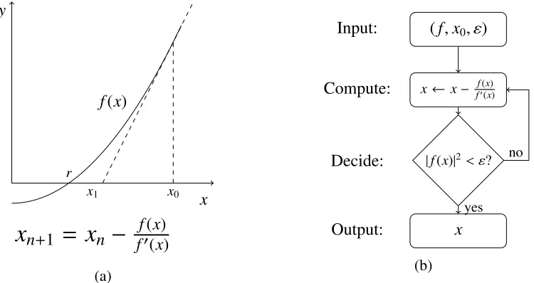
overRandC(e.g., that the Mandelbrot set is undecidable overR). Figure 1.1 shows an example
6I borrow this name from Feferman (2013).
y
f(x)
r
x
x1 x0
x
n+1=
x
n−
f(x)f0(x)
(a)
(f,x0, ε) Input:
x← x− f(x)
f0(x)
Compute:
|f(x)|2< ε?
Decide:
x
Output:
yes no
(b)
Figure 1.1: (a) Newton-Raphson method for approximating a root of f(x). (b) A BSS program implementing the method
of how Newton’s method (perhaps the most standard algorithm in Numerical Analysis texts)
is naturally captured by this model (see also Blum et al., 1997, 10). A crucial idealisation that
Blum et al. employ, though, is that the machineMis able to manipulate theexact valueof any
real number it operates on. Real numbers are viewed as whole entities and algebraic operations
and comparisons are each counted as one unit of work; that is, it always takes one step to add,
subtract, multiply, divide, and compare two real numbers, even if they are irrationals. This is not
physically possible to implement though, and thus much of the criticism directed at the model is
based on that fact. We’ll say more about this in due course.
1.3.2
E
ff
ective Approximation
As we have already said, other mathematicians have been in the business of extending Turing
computability to the domain of the reals, almost since the early 50’s. Although there is no
universally accepted formalisation of the notion of effective computation of a real-valued function, most models are for the most part equivalent, regarding their theoretical results.
It is not possible to try even a brief exposition of the different approaches here. We will only give the basic flavour of some main characteristics. For further details, a now standard reference
text is Weihrauch (2000). Friendly short expositions can also be found in Braverman and Cook
(2006) and P´egny (2016).
The main problem facing us when we move from computing over the integers to computing
since a computing agent (Turing machine or other) actually manipulates symbols from a finite
alphabet. Nevertheless, when we move to an uncountable domain, such asR, we still have
only countably many names available to denote uncountably many entities. This creates thorny
conceptual problems.
Effective approximation tackles this problem by positing that instead of the exact values of the reals, the computor deals with sequences of rationals approximating those values. Intuitively,
a function is computable if, given a “good” rational approximation of the input, there is an
algorithm that yields a “good” rational approximation of the output. Suppose a real number
xand that we want to compute f(x). Since xis a real number, there is a Cauchy sequence of
rationalshrkik∈N which approaches xas its limit. Now, to compute f(x) means to effectively
determine another rational sequencehrmim∈Nthat approaches f(x) as its limit.
Following are some different formalisations of the above intuitive idea.
The Grzegorczyk/Pour-El & Richards approaches We say that:8
• Asequence of rkrational numbers is computable, if there exist three recursive functions,
a,b,s:N→Nsuch that, for allk,b(k), 0 and
r(k)= (−1)s(k)a(k)
b(k)
• Asequence of rk rational numbers effectively convergesto a real number x, if there exists
a recursive functionn:N→N, such that for allm:
k>n(m) implies |x−rk |62−m
• Areal number is computable, if there exists a computable sequencerkof rational numbers
that effectively converges to x.
• Afunction f :I →R(where the endpoints ofIare computable reals) iscomputableiff:
– f issequentially computable: ifxiis a computable sequence of points inIconverging
tox∈I, then the sequence f(xi) is computable and converges to f(x).
– f iseffectively uniformly continuous: there exists a recursive functiond :N→ N such that for allx,y∈I and for alln∈N,
| x−y|6 1
d(n) implies | f(x)− f(y)|62
−n
The above definition is actually due to Grzegorczyk (1955). It can be seen as formulating
effective versions of the usual definitions in real analysis.
Another approach is due to M.B. Pour-El and Caldwell (1975), suggested by the Weierstrass
approximation theorem, which states that every continuous function f : [a,b] → R can be
approximated by a sequence of polynomials pn(x) overQwith non-zero rational coefficients.
The effective version of this is as follows.
A function f on a domain Iiscomputableif there exists a computable sequence of rational
polynomials pk(x) which effectively converges to f; that is, if there exists a recursive function n:N→N, such that for allmand all x∈I:
k>n(m) implies | f(x)− pk(x)|62−m
This can be extended over the wholeRas well (see, Pour-El and Richards 1989, ch.0).
This model is provably equivalent to the previous one, on any closed intervalIand onR.
Type-2 Theory of Effectivity (TTE) A different formalisation of computable functions is in terms of Turing machines.9 Here, the basic assumption is that if the output value is one
that requires an infinite string of symbols in order to be represented, then the Turing machine
computing the function, yields a (series of) approximating representations of it. The following
formalisation is due to Weihrauch (2000).
More precisely, in classical computability theory, Turing computation of a numerical function
f :⊆ Nn→ Nis expressed as computation of string functions f :⊆ (Σ∗)n →Σ∗, whereΣ∗is the set of all finite words over a non-empty finite alphabetΣ. Computability of other sets of objects (rational numbers, graphs, etc.) becomes possible by means of number coding. Nevertheless, sinceΣ∗ is actually a countable set, the above formalisation is not adequate for dealing with
computability over uncountable domains, such asR. Therefore, we also consider the setΣωof infinite sequences of symbols fromΣ.10
9Commonly referred to as ‘Type 2 Turing machines’. If we see natural numbers as type 0 objects, and reals as
functions mapping naturalsnto rationalsrn(i.e., type 1), then a real function is actually a functional, mapping functions to functions; hence, it can be seen as a type 2 object. Accordingly, effective computability over the reals is referred to as ‘Type 2 Effectivity’ (TTE).
10Σωhas the same cardinality as
For k > 0 and Y0,Y1, ...,Yk ∈ {Σ∗,Σω}, a string function f :⊆ Y1×...×Yk →Y0 is com-putable iff there is a Type-2 Turing machine M with k input tapes such that: given input (y1, ...,yk) with each (finite or infinite) sequenceyi ∈Yi written on theiinput tape, the machine
outputs ay0∈Y0, such that one of the following two cases holds:
1. fM(y1, ...,yk)=y0 ∈Σ∗andMhas halted.
2. fM(y1, ...,yk)=y0 ∈Σω, Mcomputes forever and writesy0on the output tape.
A Type-2 Turing machine M is a Turing machine with k input tapes together with a type
specification (Y1, ...,Yk,Y0) withYi ∈ {Σ∗,Σω}which gives the type for each tape. If M
com-putes forever but writes only finitely many symbols on the output tape, fM(y1, ...,yk) is undefined.
The above is a theoretical model. Infinite strings and infinite computations cannot be written and
completed in reality. However, the notion of ‘effectivity’ implies that an effective computation must be able to terminate after a finite number of steps. To alleviate these concerns, we add the
extra restrictions that the input and output tapes are one-way read-only and one-way write-only
(no written symbol can be erased). These restrictions guarantee that after some finite number
of steps, M will have read some finite initial part of the inputs and will have written some
finite initial part of the output. Additionally, the requirement of one-way output guarantees that
whatever has been written on the output tape, afterfinitelymany steps cannot be erased and is, thus, a correctprefixof y0 ∈Y0. Then, the infinite computations of Type-2 machines can be
approximatedby physical computations with arbitrary precision (Weihrauch, 2000, 16).
Ker-I Ko’s approach Another route to alleviate concerns about the theoretical idealisation of case 2 above, and tie Turing machines to physically implementable real computation, is
to restrict the input strings toyi ∈Yi whereYi = Σ∗ only and equip the Turing machine with
an oracle (see, Ko 1991). An oracle is a kind of “black box” that, at any given step of the
computation, can be queried by the TM to provide the value of a functionφ : N → Σ∗, in
one step. A machine with an oracle is a TM with input and output tapes and with one extra
distinguished tape —called ‘the query tape’— on which a statement ‘call oracle’ can appear
arbitrarily often. Whenever the machineM reaches this statement, it replaces in one step the
current wordw written on the query tape withφ(|w|).11 According to Ko’s formulation, real
numbers are represented asCauchy functionsand, so, the computing machine Mis an oracle
TM mapping Cauchy functions to Cauchy functions.
Here is an informal presentation of this approach put to work (we skip a formal treatment, which would be in terms of Cauchy functions, in the interests of brevity). Suppose that for
somexwe want to compute f(x), where f :⊆ R→ R. The trick is to work with (a series of)
approximations of the inputs and outputs to effectively computable precisions.
• We give as input to machineMthe integernsuch that the outputy0must be within the
error 2−n; that is,|f(x)−y
0|62−n.
• Mcomputes the integerm, such that 2−mis the required precision of the inputy1; that is,
|x−y1|62−m.
• Now,Mrefers to the oracle to obtainy1; that is, the oracle computes in one stepy1 =φ(m) such that|x−φ(m)|62−m.
• Mcomputesy0.
The running time of Mis the time taken to computemfromnplus the time taken to compute
y0 fromy1 =φ(m). Crucially, all these havefiniterepresentations. Thus, the computation of f :⊆ R→ Rdoes not require reading/writing of any infinitely long strings or an infinite number of steps, according to this approach.
The machine M is said to compute f iff, given that the resultφ(m) is a Cauchy function for x ∈R, and on input0m, the output is a Cauchy function for f(x) (for allx ∈dom(f) and φ:N→Σ∗).
Generalization to multivariate functions f :⊆ Rk →
R is straightforward, by allowingk
oracles,ϕ1(m), ϕ2(m), ..., ϕk(m) that can be queried with respect tom.
All the above models are, as already mentioned, virtually equivalent with respect to their
results; for example, which functions over the reals are computable.12 They also are all based
on the (independent) work of Grzegorczyk (1955) and Lacombe (1955); though, the earliest
work in this area goes back to 1937-1939, done by Banach and Mazur, but published several
decades later (Mazur, 1963) owing to WW2. Nevertheless, the groundlaying work is definitely
again Turing’s (1936). For a thorough and illuminating examination of the development of computable analysis, from Turing’s seminal work to this day, see Avigad and Brattka (2014).
1.3.3
Incompatibility between the two main approaches
There is a clear sense in which the two main approaches are incompatible. Almost all of the
functions characterized as computable by BSS are non-computable by Effective Approximation (EA), and vice-versa (see, also, Weihrauch 2000).
More precisely, a major result, which holds in all EA models, is the following:
12However, the presentation here is by no means exhaustive. See Weihrauch (2000, ch.9), for other approaches,
Any computable function is continuous.
We have already seen a version of this before (p.8), in Grzegorczyk’s definition of
com-putable functions where any such functions were required to beeffectively uniformly continuous. Although in Grzegorczyk’s definition the continuity property is obtained by fiat, as part of
the definition, in Weihrauch’s model it is a consequence of the requirement that whatever is
written on the output tape of a Type-2 TM is already a correct prefix of the output and cannot be erased. Thus, any finite portion of the output is already determined by a finite portion of
its input (Weihrauch 2000, Th.1.3.4 and 4.3.1). Intuitively, this holds because if, say, we’re
computing an approximation to a value f(x), we want this approximation to be a good one for
all points nearx, since the latter is also given by an (arbitrarily precise) approximation.
A brief comment on the continuity result. One can notice the striking similarity between the
continuity requirement in computable analysis and in constructive mathematics. In the latter too,
every real valued function is continuous at every point at which it is defined. And one cannot
always separate any two real numbers, since in some cases that might require an infinite amount of information, about one or both numbers. Thus, the following statement doesnotalways hold
for any two realsx1,x2 ∈R:
x1< x2orx1 > x2or x1= x2 (1.1)
Owing to the facts that (a) the father of intuitionism, Brouwer, held the continuity requirement
to be true13 and, (b) Borel (1912) had held a similar view even earlier, in his discussion about computable real numbers and functions, Myrvold (1995) calls this requirement ‘the
Borel-Brouwer Thesis’.
Similarly to constructive mathematics, (1.1) does not always hold in EA models either. The
equality relation and comparisons are in general non-computable.
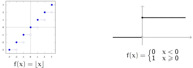
In the BSS/Real RAM approach, on the other hand, there’s no similar continuity require-ment. That means that functions seemingly easy to define, such as step or floor/ceiling functions, are not EA-computable.14 See Fig.1.2.
Furthermore, since the comparison operation is discontinuous, almost every non-trivial
branching node in the program of a BSS machine introduces a point of discontinuity. Thus,
most BSS-computable functions are non-continuous and, so, non EA-computable. Conversely,
13In fact, for intuitionists a stronger result holds: any continuous real valued function on a closed interval is
uniformlycontinuous.
14More precisely, computation of these functions becomes harder the closer we get to the discontinuity point and
Figure 1.2: A floor and a step function. Functions with discontinuity points are not EA-computable everywhere.
functions such as square roots or exponentials are not BSS-computable, whereas they’re
un-problematic for EA.15One can build such functions into a BSS machine’s program as primitive
operations, but this does not really address the problem, since there would still remain EA-computable functions (e.g., transcendental ones) that are not BSS-EA-computable.
This, creates a strong incompatibility between the two main approaches. One might even argue that they in fact are incomparable; they cannot be compared because they fulfil different purposes.16
While, indeed, the two approaches are meant to serve different purposes in general, there are however two particular aims they share in common. First, they both claim to provide,
among other things, a foundation for scientific computing. Blum’s (2004) short and very clear
exposition of the BSS model in the Notices of the American Mathematical Societyaims to
draw attention on the model as a foundation for numerical analysis and computational science.
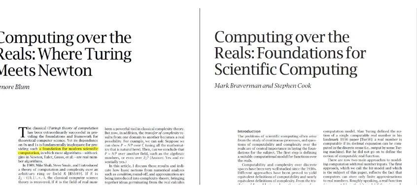
Nevertheless, two years later, again in theNotices of the AMS, Braverman and Cook (2006)
presented a version of an EA-model (under the name ‘bit computation’) as a better foundation
for scientific computing; a main point being there that their version tracks and approximates
how real computers actually compute better. See, Fig.1.3.
15Almost all of the commonly encountered continuous functions in analysis are EA-computable, on an
appro-priate domain, including, for example, f(x1, ...,xn)=c, f(x1, ...,xn)=xi, polynomials, trigonometric functions,
min(x1,x2), max(x1,x2), 1x,ex, n
√
x,|x|, etc. (see, Weihrauch, 2000).
16P´egny (2016), for example, argues that the BSS/Real-RAM models are models of analog computation which
Figure 1.3: The two articles appeared in theNotices. Both models claim to offer a foundation for scientific computing.
But another purpose for both approaches is to formalise the concept of ‘algorithm’. In the tradition of logic and computer science, effective computation of a function was always understood as computation by following an algorithm. But numerical analysis, being a centuries
old field —concerned with mechanical methods for tackling various problems such as, solving
linear or differential or integral equations, data interpolation, optimization problems, etc.— also has the notion of ‘algorithm’ at its core. Therefore, although the task of choosing among the
various theories of real computation is important on its own, I think that the very existence of
Algorithms
As we have said, ‘algorithm’ is a central concept in numerical analysis, as a long-standing
field concerned with methods for numerical problem solving. No wonder then that a formal
theory aiming to offer a foundation for the field would also claim that it formalises the notion of ‘algorithm’:
The situation in numerical analysis is quite the opposite. Algorithms are primarily
a means to solve practical problems. There is not even a formal definition of algorithm in the subject. [..]
[But a]s long as the computer is seen simply as a finite discrete object, it will be
difficult to systematize numerical analysis. We believe that the Turing machine as a foundation for real number algorithms can only obscure concepts. (Blum et al.,
1997, 23)
And, after having sketched the BSS model, Blum et al. continue:1
Now formulating a theory of computation [over a field K and choosing K to be
the real numbersR..], we are able to obtain a setting that provides a foundation
of numerical analysis. The notion of an algorithm overRbecomes well-defined
as a mathematical object in its own right. So we have developed anextensionof
the classical theory to a new theory which can be specialized to the study of real number algorithms. (Blum et al., 1997, 30, emphasis in original)
The contrast of this “opposite situation”, in the first quote, is with the case of classical
com-putability theory. As we have already mentioned earlier (p.4), the Church-Turing thesis is almost universally accepted as a foundational principle for computer science. The groundbreaking
1See, also, the quotes on p.5.
work by logicians back in the 30s, and later, successfully captured (extensionally) the notion of
an ‘effective procedure’. But saying that ‘a function is effectively computable’ can be translated as ‘there is a sequential algorithm for computing this function’. So, it is generally asserted
that the aforementioned logicians’ work successfully captured (extensionally) the notion of ‘a sequential algorithm such that..’.
But, this formal work is just as naturally extended to real function computability by the
effective approximation approaches. So it seems equally natural to consider that the notions of ‘effective computation of a real function’ and ‘sequential algorithm for computing a real function’ are suitablyexplicated by some strand from the effective approximation cluster of approaches, say, Type-2 Turing machines. And, indeed, EA is widely accepted as the correct
framework for formalising real computability, within certain fields such as logic, theoretical
computer science, physics, and also philosophy.2
Nevertheless, Blum et al. are by no means the only mathematicians complaining about
how unnatural the effective approximation models are for providing a foundation for certain mathematical fields. Researchers from the area of computational geometry have expressed
similar complaints and one of the ground-laying texts in the subject (Preparata and Shamos,
1985) uses the Real-RAM model as a formal foundation of geometric algorithms.3
Even more, information-based complexity uses Real-RAM as the standard model of
com-putation for the analysis of algorithms. Hopefully, the reader will excuse a brief digression, in
2For an insightful defence of EA as the appropriate framework to formalise effectivity, see P´egny (2016). 3Here is a rather long but very characteristic quote, distilling the attitude of researchers in computational
geometry towards effective approximation (emphasis in original):
Most (classical) results in computational geometry are heavily tied to issues in combinatorial geometry, for which assumptions about coordinates being integral or algebraic are (at best) irrelevant distractions. Speaking as a native, it seems completely natural to considerarbitrarypoints, lines, circles, and the like asfirst class objectswhen proving things about them, and therefore equally natural when designing and analyzing algorithms to compute with them.
For most (classical) geometric algorithms, this attitude is reasonable even in practice. Most algo-rithms for planar geometric problems are built on top of a very small number of geometric primitives: Is pointpto the left or right of pointq? Above, below, or on the line through pointsqandr? Inside, outside, or on the circle determined by pointsq,r,s?
[...] For similar reasons, when most people think about sorting algorithms, they don’t carewhat they’re sorting, as long as the data comes from a totally ordered universe and any two values can be compared in constant time.
So the community developed a separation of concerns between the design of real geometric al-gorithms and their practical implementation; [...] TTE, domain theory, Ko-Friedman, and other models of “realistic” real-number computation all address issues that the computational geometry community, on the whole, just doesn’t care about.
order to discuss how the Real-RAM model is employed in those disciplines (the latter using the
name ‘real number model’).
2.1
The BSS
/
Real-RAM in other areas of mathematics
Computational geometry. Computational geometry is concerned with the study of algo-rithms for solving geometrical problems, which, in a sense, are the computational counterparts
of rule-and-compass constructions of classical geometry. The latter field had been profoundly
influenced by developments in real analysis, for example, metric spaces and convexity theory.
Due to these developments, the treatment of classically geometrical notions, such as distance or
convexity, was transformed to treatment of analytic notions, such asmetricsor properties of
finitesubsets. Accordingly, the objects considered in the descendant field of computational
ge-ometry commonly are sets of points (x1,x2, ...,xk), wherexireal, in ann-dimensional Euclidean
spacewith metric (Pn i=1x2i)
1/2.
Computational geometry involves two fundamental elements,algorithmsanddata structures.
The formulation and analysis of the algorithms —e.g. their cost— is with respect to some specific
computation model. Data structures are ways of organizing the complex objects manipulated by
the algorithms —most commonly, sets, ordered and unordered— by means of the simpler data
types directly representable by the computer.4
In order for an appropriate model of computation for a mathematical domain to be chosen, the
nature of problems dealt with in the domain is essential. Generally speaking, in computational
geometry most problems can fit into one of the following categories.5 (a) Subset selection: given a collection of objects, find a subset that satisfies a certain property (e.g., the two closest ones in
a set ofnpoints). (b) Computation: Compute the value of some geometric parameter of a given
set of objects (e.g., the distance between a pair of points). (c) Decision: with any instance of the
above two categories, we can also associate a decision problem, with a YES/NO answer (e.g., does a specific subsetS satisfy propertyP? Is the distance between points A and B greater or
4Data structures can be classified according to what operations they involve. For example, ifS is a subset ofA,
represented in a data structure, anduan arbitrary member ofA, the fundamental operations are: MEMBER(u,S): Decide whetheru∈S
INSERT(u,S): AddutoS. DELETE(u,S): RemoveufromS.
Assuming now a collection of disjoint setsS1,S2, ...,Sk, more complex operations can be: FIND(u): Reporti:u∈Si
MIN(S): Report the minimum element ofS (S is totally ordered).
Accordingly, data structures are classified on the basis of supported operations. For example, a Dictio-nary, is a data structure supporting MEMBER, INSERT, DELETE, and a Priority queueis a data structure supporting MIN, INSERT, DELETE (Preparata and Shamos, 1985).
equal to a fixed constantk?).
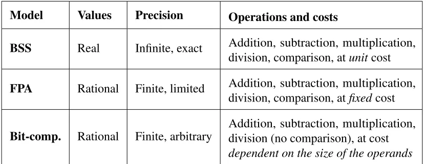
The adopted model is, as we have said, Real-RAM, which is essentially equivalent to BSS in
the finite-dimensional case. A real-RAM machine is aregister machine, but capable of storing
the exact value of a real number in each memory cell (register).6 The inputs to the machine
are unanalysed entities in an algebra A, making it an algebraic approach, similarly to BSS.
Thus, the four arithmetical operations (±,×,÷) as well as comparisons between any two real
numbers (<,6,=) are primitive and availableat unit cost. Relative to specific applications, several analytical functions, such as n-root, trigonometric ones, etc., can be taken as primitive
and built into the model.
When a real-RAM executes an algorithm for a decision problem,7 the overall computation may be viewed as a path in a rooted binary tree, whose particular nodes involve either a
calculation, or a branching based on the result of a comparison. Such a tree corresponds to
another computational model, the “algebraic decision tree”. This is an important fact, because
the worst-case running time of a real-RAM program will be at least proportional to the length
of the longest path from the root (representing the initial step of the computation) to a leaf
(representing a last step and containing a possible answer YES/NO output), in the respective algebraic decision tree. Thus, the Real-RAM model and its connection to algebraic decision
trees are very useful for analysing algorithms in terms of lower bounds of their costs.
Information-based complexity (IBC). Information-based complexity is the branch of computational complexity that studies the complexity of problems in which information is
partial,noisy, andpriced. ‘Information’ in this context is not meant in the same sense as in
Claude Shannon’s information theory. It rather is about what we know about the problem whose
complexity and solution we’re interested in. More often than not, information is limited in a
variety of problems, from science and engineering to economics and mathematical finance, to
control theory, to computer graphics and vision, etc. Assume, as a toy example, that we need
to computeR01 f(x)dx. Very often, we cannot apply the fundamental theorem of the calculus,
and we have to numerically approximate the solution (Traub et al., 1988). All we can do is to input in the computation the value of f at certain points (perhaps, obtained by some program
calculating f(x)) and this is the available information. It ispartial, since there is in general an
infinite number of integrands having the same values at these points, and our case cannot be
distinguished from any of those; we have limited knowledge only. If we also have round-offor representation errors (e.g., owing to use of a digital computer), then the information isnoisyor
contaminated. Both incompleteness and contamination of information bring about an intrinsic
6‘RAM’ stands for ‘Random Access Machine’, which is another name for register machines.
uncertainty in the answer, sayε. In addition, it is assumed that information ispriced: there
is a cost for every piece of information we obtain (e.g., in the previous example, for every
value of f(x) at a point). All such cases are contrasted with problems studied incombinatorial
complexity where information is complete, exact, and free, such as the travelling salesman problem. Typically, the way this problem is studied in combinatorial complexity is by assuming
that all the cities and all the distances between them are known completely, exactly, and with no
cost.
Similarly to combinatorial complexity,8 information-based complexity deals with the study
of all possible algorithms for solving a problem, in order to evaluate its complexity, in a way
that the latter will be a problem invariant, that is, independent of any particular algorithm used.
Since problems studied in IBCex hypothesican only be solved approximately, it is required that
a solution will not have error greater than a thresholdε. Then, theε-complexity of a problem is the minimal cost among all algorithms which solve the problem with error at mostε(Traub
et al., 1988, 3). Accordingly, the cost and error of algorithms are defined according to three
different settings: aworst case, anaverage, and aprobabilisticsetting.
The model of computation used in IBC, in order to analyse algorithm costs and, hence,
complexity of problems, is called ‘Real number model’ and it’s equivalent to BSS/Real-RAM. The crucial assumption is, again, that the four arithmetic operations and comparisons between
real numbers are primitive and that they can be performed exactly and at unit cost.
Other fields Finally, besides numerical analysis, computational geometry and information-based complexity, the Real-RAM/BSS model has been used in the field ofcomputer algebra
and mainly inalgebraic complexity. The concern here is with algorithmic problems which can
be solved by means of algebraic algorithms (B¨urgisser et al., 2013).
2.2
The problem about algorithms
So it becomes apparent that although ‘algorithm’ is the central notion in various areas of
mathematics, it is however treated and formalised differently. Nevertheless, if all mathematicians sat around a table, so to speak, they would all agree, at an informal level, about what kind of
routines qualify as algorithmic ones and what features such routines should have. And, in a
sense, this is what has been done for centuries, when the intuitive notion of ‘algorithm’ was
taken as clear and unproblematic and with no actual need for further formalisation. But, then,
8Very often and in many contexts, what we refer to here by ‘combinatorial complexity’ is just called
despite any intuitive consensus, mathematicians from different fields actually end upexplicating
the informal idea in not only different but actually incompatible ways. How can this be so?
2.2.1
Three levels of formalisation
Smith (2013, 44-45) distinguishes three levels of conceptualisation in play, when we come to
formalise intuitive concepts. I will adopt his scheme for the purposes of this work and with respect to the notions of ‘computation’ and ‘algorithm’.
First, we can say that there is apre-theoretic level, at which the basic notion of
‘computa-tion’ is actually a vague, rough idea, stemming mainly from paradigmatic cases of algorithmic
procedures in the mathematical practice (e.g., the sieve of Eratosthenes or Euclid’s algorithm).
The ideas are still inchoate at this level and we rather have to do with a cluster of notions instead
of a simple one. There’s not one definite idea of ‘computation’ (or ’calculation’) but various
distinct cases: effective computation, machine computation, analog computation, geometric constructions, etc. All these are not excluded by any pre-theoretical talk of computation or of mechanical procedures.
Second, at a next, proto-theoretic, level, things become more specific. This is the level at
which we “tidy up” the notion by means of certain abstractions and idealisations. It is important
to stress that there may be an element of decision here, in the sense that we choose to pick up
certain strands from the pre-theoretic hodgepodge of ideas andsharpenthe particular notion.9
So, what the founding fathers of computability did, back in the 30s, was to pick out the strand
of ‘effective computation’ (i.e., computation by following a sequential algorithm) and abstract away from limitations of time and space.
It is not clear whether there is also an element of choice about exactly what idealisations to employ when sharpening intuitive notions; when Church, Turing, et al., for example, idealised
from matters of feasibility in order to formulate effective computation. After all, there are other notions of computability as well and it seems reasonable that a different mathematical community could have set, say, some fixed upper bounds to how fast a function grows, in order to
be regarded as ‘computable’, such as to be calculable in at most exponential or hyperexponential
9I should emphasize from the outset that, by saying that there is an element of decision in the above procedure,
I donotmean that the whole process of sharpening the concepts is an arbitrary one. Rather, I mean something along similar lines to Carnap’s (1962) views onexplication; namely that before we go on with our attempt to provide a satisfactoryexplicatumof the concept in hand, we need to make clear what is meant by theexplicandum. That is, we need to provide explanations of what is and what is not the intended use of the intuitive concept to be explicated; what is intended to be included and what to be excluded. For example, by wanting to explicate ‘truth’, e.g. in a Tarskian way, we specify that we mean ‘truth’ as, say, used in the sense of ‘correct’, as applied to
time, etc. See Shapiro (2013) for arguments in favour of such a view. In all those cases, functions
such as Ackermann’s would not qualify as computable (and therewerevoices at the time arguing
to that effect). On the other hand, G¨odel seemed to hold that —at least in some cases— there is only one correct way of formalising an intuitive concept; we only need to gain “the correct perspective”:
If we begin with a vague intuitive concept, how can we find a sharp concept to correspond to it faithfully? The answer is that the sharp concept is there all along,
only we did not perceive it clearly at first. This is similar to our perception of an
animal first far away and then nearby. We had not perceived the sharp concept of
mechanical procedures before Turing, who brought us to the right perspective. And
then we do perceive clearly the sharp concept.
If there is nothing sharp to begin with, it is hard to understand how, in many cases,
a vague concept can uniquely determine a sharp one without even the slightest
freedom of choice. (quoted in Wang 1997, 232-3)
We need not settle this issue here. But we will have some relevant discussion further on.
Finally, the third,fully-theoretic, level is when we have come to formulate rigorous and definite
concepts, such as those of ‘Turing computability’, ‘µ-recursiveness’, etc. The concepts now in
play are rigorously defined and precise, and little (if anything) is left to intuition. In our case, for
example, it seems reasonable to assume that were a new function (on the natural numbers) to be
discovered tomorrow, there would be a definitive answer whether it is, say, Turing-computable
or not (even if it was extremely difficult in practice to find that answer).
So, in the case of computability, the Church-Turing thesis links the extensions of the
sharpened notions at the second level (i.e., ‘effective computation’) with those of the rigorous mathematical concepts of the third level (e.g., ‘recursive functions’). And what it does is to
identify these extensions. And since effective computation is understood as computation by following an algorithm, the CTT can be seen as explicating the idea of ‘algorithmic computation’
by means of ‘Turing computation’, (or ‘recursiveness’, or whichever your preferred model is).
2.2.2
Three possible interpretations
Now, how are we to interpret the fact that although arguably all mathematicians would agree
about theproto-theoretic characterisation of ‘algorithm’, they end up formalising it, at the third
level, in incompatible ways, according to which mathematical area they come from? I suggest
A) The first possibility is that only one approach is in fact proper (or, acceptable). The
proto-theoretical notion of ‘algorithm’ is as precise as it gets for an informal concept and, despite
some vagueness in thesenseof the term —what is meant by ‘small steps’ in an algorithm, for example?—, we should always pick out the same class of algorithmically computable functions,
under any reasonable sharpening. This was the case with the numerical functions over the
non-negative integers, and it’s also the case (for the most part) with the different models within the cluster of effective approximation. Thus, effective approximation gets it right, whereas BSS/Real-RAM or other unrealistic models of computation actually miss the point.
B) The second possibility is to say that we in fact use the notion of ‘algorithm’ in mathematics
in more than one way. To make this idea more precise, let’s say that a concept ispoly-vagueif
our informal talk about it fails to pick out a single mathematical “natural kind”.10 A poly-vague term, then, can legitimately be disambiguated in more than one way, though consistently with
the implicit rules we’d mastered for applying the concept to ordinary cases.
So, following that route, we can say that in the traditions of numerical analysis and geometry
the term ‘algorithm’ picks out different classes of routines from those of computer science (though each class might be precisely bounded).
C) The third possibility is that, although already aproto-theoretical concept (that is, some
theoretic tidying has already taken place), ‘algorithm’ is a concept withopen texture. This means that the concept itself has some open-ended character in the sense that the so far established use
of the language is not adequate to delimit it in all possible directions.
The term ‘open texture’ is due to Waismann (1945), who, at the time, was arguing against
verifi-cationism, on the grounds that most (though not all) empirical concepts cannot be exhaustively
and precisely defined; there can always exist some unforeseen situations or instances falling
under their extension. This, as a fact, prevents us from conclusively verifying most of our
empirical statements. Assuming that a term is considered defined when the sort of situations in
which it is to be used are defined, empirical concepts can never be completely defined, due to an open horizon of possible situations that any empirical description might leave out. Nevertheless,
for Waismann, mathematical terms do not suffer from any similar incompleteness of definition, because a definition of, say, a geometrical term, such as a triangle, in a sense includes already
all sorts of situations in which it can be used. The description of the term is already complete.
Despite that, Stewart Shapiro, in two related articles (2006; 2013), has argued that open
texture can be a property of some mathematical terms as well; ‘number’ and ‘computable’, for
example, being cases in point.
Now, in terms of the three-level schema, described in the previous section (2.2.1), it is
safe to assume thatpre-theoretic concepts may exhibit open texture. The different notions of ‘computation’ not excluded from thepre-theoretic idea is a good example of this. What is more
contentious, though, is the claim that theproto-theoretic concept of ‘algorithm’ may still have some open texture too.
Supporters of all three interpretations (explicitly or implicitly) can be found both in
philoso-phy and mathematics/Computer Science. But before we attempt a more thorough discussion about their plausibility, we need a more ‘precise’ formulation of the informal idea of ‘algorithm’.
2.2.3
Algorithm: the informal concept
Although informal, ‘algorithm’ has always been taken as a clear and unproblematic notion.
Virtually all mathematicians would agree on something like the following features as being the
essential ones:11
1. An algorithm is a general step-by-step procedure, prescribing a sequence of operations
for solving a type of problem. It must be expressed as a set of instructions offinite size.
2. An algorithm has a set (perhaps empty) of inputs and a (set of) output(s).
3. For any given input, the computation is carried out in a discrete stepwise fashion (that is,
without use of any continuous methods or analog devices). Alternatively put, an algorithm
proceeds in discrete time, so that at every given moment the state of the computation is
obtained from the state at the previous moment of time.
4. For any given input, the computation is carried out deterministically, without resort to any
random methods. The computation state at any given step/moment isuniquelydetermined by the state in the preceding step/time and the list of instructions.
5. The list of instructions that make up the algorithm are to be followed by a computing
agent (human or otherwise) which carries out the computation.
6. Each step of an algorithm must be specified to the smallest detail, precisely and
unam-biguously, such that no acumen or ingenuity or any semantic interpretation is required by
the computing agent. Steps should be of a bounded complexity.
11The characterisation I provide here is distilled by relevant descriptions in the classic works of Knuth (1997),
Computations possessing feature (1) are sometimes called ‘sequential-time’ (as opposed,
e.g., to parallel or distributed computations). Computations with features 1 and 6 are sometimes
called ‘sequential’. Sequential algorithms are a subspecies of sequential-time ones.
The above 1-6 features are almost universally accepted as necessary. There is also the requirement offiniteness:
7. An algorithm must always terminate after a finite number of steps.
But, although many texts explicitly pose this requirement (Rogers, 1987; Knuth, 1997),
some authors may accept non-terminating procedures satisfying the above criteria as algorithms
too.12 The concern with finiteness arose in the context of effectively computing and is explicitly expressed in Hilbert’s 10thproblem, posed in 1900 at the International Congress of
Mathemati-cians in Paris: “Given a Diophantine equation [..] devise a process according to which it can be
determinedin a finite number of operationswhether the equation is solvable in rational integers”
(emphasis added). It is trivial, however, that not all processes which clearly are algorithmic can be carried out in a finite number of steps; consider the calculation of the quotient of two
incommensurable numbers, for example.
In practice, though, the process always terminates when it reaches some previously agreed
stage. Additionally, for every function which qualifies as computable, in the sense of the
existence of an algorithm for computing its values, the corresponding algorithm must, obviously,
be terminating.
2.2.4
The problem reformulated
Given the above features, a main question pursued in this chapter is this:
12For example, (Hermes, 1969, 2):
There are terminating algorithms, whereas other algorithms can be continued as long as we like. The Euclidean algorithm for the determination of the greatest common divisor of two numbers terminates; [..] The well-known algorithm of the computation of the square root of a natural number given in decimal notation does not, in general, terminate. We can continue with the algorithm as long as we like, and we obtain further and further decimal fractions as closer approximations to the root.
Or, (Gurevich, 2015, 189):
In general algorithms perform tasks, and computing functions is a rather special class of tasks. Note in this connection that, for some useful algorithms, non-termination is a blessing, rather than a curse. Consider for example an algorithm that opens and closes the gates of a railroad crossing.
Does the above informal characterisation have enough shape to pick out always
a precisely bounded class of routines/computable functions?13
If the answer is ‘yes’, then something like the (A) possibility from the previous section (2.2.2)
must be the case; if ‘no’, then either (B) or (C).
Of course, the case of classical computability theory gives strong evidence in favour of
the first option. The informal notion has throughout the history of mathematics been taken as
clear, precise, and unproblematic, and when the need for formalisation arose —in order to prove
non-existence results about algorithms—, all formal models (all attemptedexplicata, that is)
turned out to be equivalent. Hence, despite any ‘vagueness’ in the informal characterization
of ‘algorithms’, the latter does have enough shape to pick out always, under any reasonable sharpening, the same class of routines/functions, when we are in the domain of the non-negative integers. And this is also in accord with G¨odel’s view in the quoted passage (sec.2.2.1).
Nevertheless, crucially, computations do not only pertain to denumerable domains, and
we saw areas of mathematics with the notion of algorithm at their heart already. So, before
attempting an answer to the question above, we need to examine the concept of ‘algorithm’ as
occurs in such domains too. We attempt an investigation within both a historical and theoretical context.
2.3
Historical context
The word ‘algorithm’ comes from the medieval term ‘algorism’. The latter is derived from
‘Algoritmi’, the latinised version of the name of the Persian Muslim mathematician al-Khw¯arizm¯ı
(c.780–850AD) who lived and worked in the House of Wisdom in Baghdad.14 Al-Khw¯arizm¯ı’s
work is, among others, responsible for the spread of the decimal positional number system
across Europe, mainly through the translations of his books on (a) arithmetic: Kit¯ab al-Jam’
wat-Tafr¯ıq bi-H, is¯ab al-Hind (The Book of Addition and Subtraction According to the Hindu
Calculation) and (b) algebra, that is, on finding the positive roots of quadratic equations:
Al-kit¯ab al-mukhtas,ar f¯ı h,is¯ab al-˘gabr wag’l-muq¯abala(The Compendious Book on Calculation
by Completion and Balancing).15 From the time that al-Khw¯arizm¯ı’s work became known in
Europe (around the 12thcentury), a conflict between the advantages of using the new positional
13By ‘computable’ here, we only refer to those functions whose value can be computed by following an algorithm,
in the above sense.
14The shift from ‘algorism’ to ‘algorithm’ is, according to one interpretation, due to a mistaken etymological
rooting when European scholars had lost track of the correct root and attributed a Greek root connected possibly with the Greek word ‘arithmos’ (number). Another interpretation has been that ‘algorism’ comes from ‘Algorismi’ and ‘algorithm’ from ‘Algoritmi’, both latinised versions of ‘al-Khw¯arizm¯ı’.