Cover Page
The handle http://hdl.handle.net/1887/18620
holds various files of this Leiden University
dissertation.
Author
:
Tran, Minh Ngoc
Workload Modeling and Performance
Evaluation in Parallel Systems
Workload Modeling and Performance Evaluation in
Parallel Systems
PROEFSCHRIFT
ter verkrijging van
de graad van Doctor aan de Universiteit Leiden,
op gezag van Rector Magnicus prof. mr. P.F. van der Heijden, volgens besluit van het College voor Promoties
te verdedigen op donderdag 22 maart 2012 te klokke 15.00 uur
door
Trân Ngo.c Minh
Promotiecommissie
Promotoren: Prof.dr. H.A.G. Wijsho Co-promotor: Dr. A.A. Wolters
Overige leden: Prof.dr. D.H.J. Epema (Delft University of Technology) Prof.dr. K.A. Gallivan (Florida State University, USA) Prof.dr. F.J. Peters
Prof.dr. J.N. Kok
This work was funded by NWO in the project Guaranteed Delivery in Grids.
Advanced School for Computing and Imaging
This work was carried out in the ASCI graduate school. ASCI dissertation series number 255.
Workload Modeling and Performance Evaluation in Parallel Systems Trân Ngo.c Minh
Thesis Universiteit Leiden ISBN: 978-90-8891-387-7
Printed by: Proefschriftmaken.nl
Contents
1 Introduction 1
1.1 Research Statement . . . 2
1.1.1 Scheduling Problem . . . 3
1.1.2 Two Challenges in Scheduling Design . . . 3
1.1.3 Challenge from Potential Impacts of Workloads . . . 4
1.2 Related Work . . . 5
1.3 Thesis Organization . . . 7
1.3.1 Chapter Overview . . . 7
1.3.2 List of Publications . . . 10
1.3.3 Roadmap . . . 11
2 Background Knowledge 13 2.1 Background Statistics . . . 13
2.1.1 Marginal Statistics . . . 13
2.1.2 Autocorrelation . . . 14
2.1.3 Cross-correlation . . . 14
2.2 Representations of Arrival Events . . . 15
2.3 Denitions of Workload Features . . . 16
2.3.1 Features of an Arrival Process . . . 17
2.3.2 Features of Runtime and Parallelism . . . 19
2.3.3 The Bag-of-Tasks Behaviour . . . 22
ii Contents
3 Statistical Analysis 25
3.1 Workload Data under Study . . . 25
3.2 Job Arrival Analysis . . . 27
3.3 Runtime and Parallelism . . . 29
3.3.1 Runtime Classication . . . 29
3.3.2 Examination of Correlation . . . 30
3.3.3 Examination of Temporal Locality . . . 30
3.3.4 Examination of Spatial Burstiness . . . 33
3.4 Basic Analysis of Bag-of-Tasks . . . 33
3.5 BoT Arrival Analysis . . . 35
3.5.1 Interarrival Times and Temporal Burstiness . . . 36
3.5.2 Long Range Dependence and Periodicity . . . 37
3.6 BoT Size, Runtime, Parallelism and Estimate . . . 40
3.7 BoT Performance . . . 43
3.8 Importance of Workload Features . . . 44
3.9 Summary . . . 45
4 Modeling Job Arrivals 47 4.1 Theory of Multifractal Wavelet Model . . . 47
4.2 MWM and Burstiness . . . 49
4.3 Data Modeling and Synthesis of Standard MWM . . . 50
4.4 Modication of MWM . . . 51
4.5 Experimental Results . . . 54
4.5.1 Long Range Dependence . . . 55
4.5.2 Temporal Burstiness . . . 55
Contents iii
5 A Comprehensive Parallel Workload Model 57
5.1 The Comprehensive Model . . . 57
5.1.1 Runtime Classication . . . 57
5.1.2 Performance of BoTs . . . 58
5.1.3 Parallelism Classication . . . 58
5.1.4 The Complete Model . . . 59
5.2 Experimental Results . . . 61
5.2.1 Bag-of-Tasks Behaviour . . . 62
5.2.2 Spatial Burstiness . . . 62
5.2.3 Marginal Distributions . . . 63
5.2.4 Correlation between Runtime and Parallelism . . . 64
5.2.5 Simulation-Based Evaluation . . . 64
5.3 Related Work . . . 65
5.4 Summary . . . 66
6 Performance Impact of Job Arrivals on Clusters and Grids 69 6.1 Workload Models . . . 69
6.2 Realistic Simulation and Requirements . . . 70
6.3 System Scenarios . . . 71
6.4 Experimental Results . . . 71
6.4.1 Cluster Scenario . . . 72
6.4.2 Grid Scenario . . . 74
6.5 Related Work . . . 76
iv Contents
7 Performance Impact of Runtime and Parallelism on Scheduling 79
7.1 Control Correlation . . . 79
7.2 Realistic Simulation Methodology . . . 84
7.2.1 Applied Workload Model . . . 84
7.2.2 Scheduling Policies . . . 84
7.3 Experimental Results . . . 85
7.3.1 Performance Impact of Correlation . . . 85
7.3.2 Performance Impact of Locality . . . 89
7.4 Discussions . . . 89
7.5 Summary . . . 91
8 A History-Based Predictor of Parallel Application Runtimes 93 8.1 Related Work . . . 94
8.2 Workloads Under Study . . . 95
8.3 Predict Application Runtime . . . 96
8.3.1 Dene Job Similarity . . . 96
8.3.2 Predict the Runtime for a Future Job . . . 98
8.3.3 Train for Best Parameters . . . 100
8.4 Experimental Results . . . 103
8.4.1 Metrics Used in Evaluation . . . 103
8.4.2 Underestimation Problem . . . 104
8.4.3 The Mean Absolute Error . . . 105
8.4.4 The Weighted Absolute Error . . . 106
8.5 Summary . . . 107
9 Conclusions 109
Samenvatting 123
Acknowledgements 125
Chapter 1
Introduction
Parallel processing is the key to fulll high demands in large-scale computing nowa-days. Not only scientic but also industrial applications have become larger and inexecutable on a sequential computer due to time-constraint requirements. This has further pushed research in parallel computing into the mainstream, where parallel systems play a central role. They help to shorten the execution time of large applica-tions, so increase user performance. Furthermore, the role of parallel systems is more important with the emergence and the rapid evolvement of grid and cloud computing because they are used as underlying basic components in grids and clouds. The fact is that parallel systems are growing rapidly in size, showing the urgent need of large-scale parallel platforms. Using data obtained from the TOP500 Supercomputing Sites [103], Figure 1.1(a) indicates that parallel systems with less than 8K processors seem unable to satisfy user demands in recent years and so larger parallel systems have been developed as a consequence as shown in Figure 1.1(b). Along with the rapid growth of parallel systems, questions regarding their performance like how to design an ecient parallel scheduler? are always challenging issues. Although research on enhancing the performance of parallel systems through smart scheduling designs has grown since numerous decades, parallel job scheduling is still a hard research topic and far from obtaining an ecient solution in practice. Investigating the Parallel Workloads Archive [80], we see that most parallel systems nowadays still implement the simple scheduling policy First-Come-First-Served with the support of backlling despite several new scheduling policies are proposed annually [27]. Therefore, we be-lieve that research on parallel scheduling should continue actively to bring ecient solutions into practice.
2 Chapter 1. Introduction
analysis should be created. The models can help to generate as many workloads as desired. Thirdly, workload models are used in experiments to evaluate the perfor-mance impacts of realistic observed workload characteristics on schedulers. Through the experiments, a better understanding of workload characteristics is derived and useful clues can be constructed to take advantage of the characteristics for better scheduling decisions. Finally, with a good understanding of real workloads and the achieved clues, ecient scheduling policies can be designed and ideally evaluated by means of simulation before they are implemented in real systems.
93 95 97 99 01 03 05 07 09 11 0
100 200 300
Year
Number of systems
1K−2K 2K−4K 4K−8k
(a)
93 95 97 99 01 03 05 07 09 11 100
101 102
Year
Number of systems
8K−16K 16K−32K 32K−64K 64K−128K 128K−
(b)
Figure 1.1: The growth of parallel systems in terms of number of processors. Data are obtained from the TOP500 Supercomputing Sites [103].
This thesis focuses on the rst three steps while the last step is still an open question. The core of the thesis is to fully exploit workload data for performance evaluation of parallel systems. The following sections introduce the main research problem, present related work and end with the organization of the thesis.
1.1
Research Statement
1.1. Research Statement 3
1.1.1
Scheduling Problem
The term scheduling has a broad variety of meanings in parallel system performance, depending on the perspective for optimization. From the perspective of a user, it can be considered as application/task scheduling [43, 74] where the objective is to nd the best schedule for tasks of a single parallel application submitted by the user. However, this kind of scheduling does not take care of other applications running on the same system, so can potentially harm the whole system performance. This research concerns primarily with job scheduling, where the purpose is to decide when and where each job should be executed from the perspective of the system [111]. The term job refers to some application which can be either serial or parallel. The scope of this study is for rigid jobs which do not change their requested number of processors at runtime. A job consists of three attributes: the arrival time indicating the submission time of the job, the runtime indicating how long the job is executed, and the parallelism indicating how many processors the job requests. Once a job is allocated to processors, it can exclusively use the processors until its execution is complete.
The job scheduling problem in parallel systems can be described as follows. Given a parallel system consisting of N processors and a parallel workload consisting of M jobs, and assume that all of these jobs are submitted to the system for execution according to their arrival time. The scheduling purpose then is to nd an ecient schedule to allocateM jobs toN processors so that the system can obtain the maximal utilization.
There are several non-trivial challenges in the eld of parallel job scheduling [26]. This thesis does not tackle directly the scheduling problem but focuses on the key chal-lenges to reach possible optimal solution for the problem. These chalchal-lenges are raised from either the designed scheduling strategies or the designers, and are described in Sections 1.1.2 and 1.1.3, respectively.
1.1.2
Two Challenges in Scheduling Design
4 Chapter 1. Introduction
well with a trace in the future since a workload can and will evolve over time. The design of a new scheduler should be evaluated by means of simulation with hundreds of workloads to ensure good scheduling performance with future workloads. This fact leads to the urgent need of representative workload models that help to generate sev-eral synthetic workloads to fulll the requirement of the simulations. Therefore, the major challenge for scheduling evaluation is the creation of representative workload models.
In order for a good scheduling decision, useful information must be transferred to the scheduler. It is crucial that the transferred information is of high quality. One of the most important scheduling information is the runtime of a job that is estimated before execution. This information is particularly useful for backlling scheduling policies, which are implemented intensively in current parallel systems. The estimated runtime of a job can be either provided by its user or predicted automatically by the system. However, user estimated runtime is relatively inaccurate [73] and so system predictors become more favorite [70]. Hence, another challenge for scheduling design is the necessity of an ecient runtime predictor.
1.1.3
Challenge from Potential Impacts of Workloads
The two challenges described in Section 1.1.2 are related to the central role of work-loads, which leads to the next challenge in nding an ecient solution for the schedul-ing problem. It is essential for schedulschedul-ing designers to have a good understandschedul-ing of real workloads before they start designing scheduling strategies. Towards this end, several long-term parallel workloads have been collected [80] and characterized [19, 48, 51, 63]. From these analysis studies, a number of workload features1 have been found, namely periodicity, long range dependence, temporal burstiness of job arrivals, Bag-of-Tasks behaviour, spatial burstiness, temporal locality and correlation. The periodicity is observed since jobs are often submitted in cycles, in particular daily cycles. The long range dependence in a job arrival process means that successive sam-ples of the process are not independent of each other, instead they are correlated. The notion of temporal burstiness is the tendency of arrivals to occur in bursts, separated by long periods of no arrivals. The Bag-of-Tasks behaviour refers to the submission of several similar jobs within a small duration. The spatial burstiness of a parallel workload refers to the non-uniformity of the distributions of runtimes and numbers of processors. The phenomenon of temporal locality is understood as a persistent similarity between runtimes of consecutive jobs. The correlation feature refers to the cross-correlation between numbers of processors and runtimes. We refer to Chapter 2 for formal denitions of these characteristics. These workload features may po-tentially have signicant impacts on scheduling performance. A deep understanding of these features will be helpful to nd useful clues for enhancing parallel schedulers.
1The words “feature”, “property” and “characteristic” will be used interchangably with the same
1.2. Related Work 5
Therefore, the challenge question with regard to workloads that will be studied in this thesis is What are the performance impacts of workload features on parallel system scheduling?.
1.2
Related Work
be-6 Chapter 1. Introduction
cause it needs a profound analysis and understanding of real world data. It is even more dicult if one wants to incorporate several workload properties into a model simultaneously. Current models [8, 18, 39, 40, 59, 95] can only capture from zero to at most two workload characteristics. As a matter of course, the more characteristics a model can capture, the more representative it is. This is also the advantage of our study since we provide a realistic model that incorporates up to ve important workload properties at the same time, as is introduced and elaborated later in Section 1.3.1 and Chapter 5.
With respect to research on performance evaluation, though several workload fea-tures are considered to be present commonly in real data and they certainly have potential impacts on scheduling, these performance impacts are hardly described in the literature. We know about only four performance studies on workload features [22, 39, 46, 57]. In [39] performance issues of the Bag-of-Tasks behavior are described. The scheduling eect of daily cycles of activity is investigated in [22]. The correlation feature is studied in [57] while long range dependence is researched in [46]. It should be noted that these studies only focus on the performance of single workload feature with an assumption about the absence of the other ones. Therefore, the question of What are the combined impacts of workload features on scheduling performance? is still open. Furthermore, the performance of several workload properties such as temporal burstiness and temporal locality is still not known.
1.3. Thesis Organization 7
the temporal locality and the cross-correlation between runtimes and parallelisms as well as the performance interaction between them.
1.3
Thesis Organization
This thesis consists of nine chapters. Beside Chapter 1 presenting the introduction, the other eight chapters are described in this section. In addition, we provide a list of publications that are connected to each chapter and a roadmap to instruct the reader an easy way to read the thesis.
1.3.1
Chapter Overview
The following paragraphs summarize the remaining chapters of this thesis:
Chapter 2 introduces necessary background knowledge and technical terms used in this thesis. The provided background knowledge includes the denition and the dif-ferent representations of arrival events. Basic statistical and probability measures are presented such as distribution functions, rst order statistics and correlation functions. In addition, several important features of a point process such as periodicity, long range dependence, temporal and spatial burstiness, temporal locality, (auto/cross)-correlation, etc. are also presented. These features play a crucial role where the research as described in this thesis centers around.
8 Chapter 1. Introduction
Chapter 4 proposes a model for job arrivals, which is an essential part of parallel workload modeling. Although a job arrival process has many important character-istics such as long range dependence and temporal burstiness, in many studies, it is assumed to be a Poisson process in evaluation work, for simplicity. Since these two characteristics may potentially aect the performance evaluation process, we argue that any job arrival model should take them into account to make itself more realistic. Despite the fact that there are several studies which model long range dependence for an arrival process, most of them focus only on network trac and less on system job trac. Furthermore, to our knowledge, there is currently almost no research focus-ing on both long range dependence and temporal burstiness at the same time. With respect to this research trend, the multifractal wavelet model [85] recently has been introduced as a good choice to yield long range dependence for a job arrival process. Though long range dependence is well captured, we observe that a job arrival pro-cess produced by this model does not keep temporal burstiness. In this chapter, we present our study on modifying the multifractal wavelet model to adapt it to system job trac so that not only long range dependence but also temporal burstiness are produced in a synthetic job arrival process that is generated by the adapted model.
Chapter 5 suggests a comprehensive realistic model for parallel system workloads, which is developed from the job arrival model proposed in Chapter 4. A job generated by this comprehensive model consists of three attributes, namely the arrival time, the runtime and the parallelism. Several statistical studies [18, 19, 48, 51, 56] have shown that the characteristics of parallel system workloads are far from independently dis-tributed. Instead, they have numerous important and correlated characteristics such as the cross-correlation between runtime and parallelism, spatial burstiness, Bag-of-Tasks behaviour, etc. All of these properties may have signicant impacts on the scheduling performance of parallel systems. In fact, there are many studies on pro-viding workload models to capture these properties [19, 39, 45, 59]. However, these studies only capture each characteristic separately and ignore others. Therefore, using these models in evaluating scheduling algorithms will lead to potentially inaccurate results because the impact of the interactions among the characteristics are neglected. Hence, we argue that a workload model should incorporate as many realistic work-load properties as possible. The comprehensive and realistic model we propose in this chapter will concurrently capture several important characteristics of parallel sys-tem workloads including 1) long range dependence, 2) sys-temporal burstiness, 3) spatial burstiness, 4) Bag-of-Tasks behaviour, and 5) correlation between runtime and num-ber of processors. This model is comprehensive and highly realistic, compared with current workload models in the literature, because it can capture up to ve realistic workload features at the same time and covers three workload attributes that are essential for simulation of schedulers.
charac-1.3. Thesis Organization 9
teristics to drive simulations of realistic system scenarios. Our experiments show that background workloads with long range dependence and temporal burstiness struc-tures cause a performance degradation of a cluster but seem to have little impact on a grid. In contrast, grid workloads with these properties do not aect the scheduling performance of a cluster but decrease that of a grid. Furthermore, we also indicate that using workloads with/without these features in evaluating cluster schedulers may produce dierent results.
Chapter 7 investigates the scheduling performance of parallel systems under var-ious patterns of parallel workloads, namely those with the two features of temporal locality and correlation between runtime and parallelism. Feitelson [18] recently indi-cated that temporal locality is a newly identied phenomenon in parallel workloads and it is essential to investigate its eects on parallel systems. According to our knowledge, there are few studies on the impacts of the temporal locality and corre-lation features on scheduling performance. Since these impacts are not well known, scheduling algorithms are often evaluated with random workloads, which neglect the phenomenon of temporal locality and the correlation. Because our study shows that these two features can signicantly aect the performance of schedulers, this can result in an inaccurate scheduling evaluation for parallel systems. In our simulation-based experiments, an increase of the correlation can quickly degrade the parallel system performance and can change the result of comparing dierent scheduling poli-cies. With respect to temporal locality, we indicate that this feature does not always seriously aect schedulers of parallel systems, but in particular situations, it can help to improve scheduling performance. Furthermore, we also discuss in this chapter the necessity of using workloads with these features in scheduling evaluation as well as how to utilize the features to enhance the performance of schedulers.
Chapter 8 presents a novel method to predict job runtimes on backlling paral-lel systems. Backlling algorithms [73] have become more popular for scheduling in many space-shared computing resources nowadays. With backlling, an estimate of job runtime is necessary for each job to determine whether it is short enough to be backlled. The estimate can be either provided by the user or predicted automati-cally by the system. However, the user estimated runtime is found to be extremely inaccurate [73] and therefore ecient system predictors for job runtimes should be developed. The predictor proposed in this chapter is based on mining historical data to obtain important parameters. These parameters are then applied to predict the runtime of future applications. It has been shown in previous works [73, 108] that both underestimation and inaccuracy in prediction have adverse impacts on schedul-ing performance of backllschedul-ing systems. In this study, we try to reduce the number of jobs that are underestimated and reduce the prediction error as much as possi-ble. Comparing with other predictors, experimental results show that our predictor is upto 25% better with respect to the problem of underestimation. Moreover, using the metric proposed in [108] for the accuracy, our predictor improves upto 32%.
10 Chapter 1. Introduction
grids. The chapter nalises this thesis by suggesting some open questions for future research.
1.3.2
List of Publications
The following list of peer-reviewed papers are connected with research chapters in this thesis:
Chapter 3
• T. N. Minh, L. Wolters, Towards a Profound Analysis of Bags-of-Tasks in Paral-lel Systems and Their Performance Impact, International ACM Symposium on High Performance Parallel and Distributed Computing (HPDC), pp. 111-122, 2011.
Chapter 4
• T. N. Minh, L. Wolters, Modeling Job Arrival Process with Long Range De-pendence and Burstiness Characteristics, International Symposium on Cluster Computing and the Grid (CCGRID), pp. 324-330, 2009.
Chapter 5
• T. N. Minh, L. Wolters, D. Epema, A Realistic Integrated Model of Paral-lel System Workloads, International Conference on Cluster, Cloud and Grid Computing (CCGRID), pp. 464-473, 2010.
• T. N. Minh, L. Wolters, D. Epema, A Systematic Approach for Parallel Work-load Modeling, Annual Conference of the Advance School for Computing and Imaging (ASCI), 2010.
• T. N. Minh, L. Wolters, Modeling Parallel System Workloads with Temporal Locality, Job Scheduling Strategies for Parallel Processing (JSSPP), LNCS, vol. 5798, pp. 101-115, 2009.
Chapter 6
• T. N. Minh, L. Wolters, Performance Impact of Job Arrivals on Clusters and Grids through Realistic Model-Based Simulation, International Sympo-sium on Performance Evaluation of Computer & Telecommunication Systems (SPECTS), pp. 22-29, 2011.
1.3. Thesis Organization 11
• T. N. Minh, L. Wolters, Model-Driven Simulation to Evaluate Performance Impact of Workload Features on Parallel Systems, International Conference on Cluster Computing (CLUSTER), pp. 84-92, 2011.
Chapter 8
• T. N. Minh, L. Wolters, Using Historical Data to Predict Application Run-times on Backlling Parallel Systems, International Conference on Parallel, Distributed and Network-Based Processing (PDP), pp. 246-252, 2010.
In addition to the above publications, a journal paper has been submitted:
• T. N. Minh, D. Epema, L. Wolters, Analysis and Modeling of Parallel Work-loads with Realistic Characteristics, IEEE Transactions on Parallel and Dis-tributed Systems (TPDS), 2011. (submitted)
1.3.3
Roadmap
12 Chapter 1. Introduction
Chapter 2
Background Knowledge
This chapter provides basic theories used in workload characterisation and modeling such as statistical knowledge and methodologies. Throughout this thesis, the chapter should be the rst choice of reference for the reader, where further references will be given for deeper understanding. The chapter starts with basic statistical measures such as distribution functions, rst order statistics and correlation functions. Then, dierent representations of arrival events are introduced. Finally, denitions of impor-tant characteristics of point processes are presented, which play a central role in the research target of later chapters. They serve as research methodologies in workload analysis and as the objectives that workload models should capture.
2.1
Background Statistics
This section covers some background concepts used in the statistical analysis of point processes. Since these concepts are presented in brief, we refer readers to [4, 19, 47, 86] for more information about these basic measures.
2.1.1
Marginal Statistics
LetX={Xn}be a stochastic point process. We present in this section some marginal
properties of X, including mean µ, variance σ2, standard deviation σ, coecient of variationCv, cumulative distribution function (CDF) F(x), and complementary
14 Chapter 2. Background Knowledge
The CCDF is opposite to the CDF and is used to answer the question how often the random variableX is above x. All of these marginal properties are calculated as
• meanµ=
Pn
i=1Xi
n , • varianceσ2=Pni=1(Xi−µ)2
n−1 , • standard deviationσ=
qPn
i=1(Xi−µ)2
n−1 , • coecient of variation Cv=σµ,
• CDFF(x) =P{X ≤x},
• CCDFF0(x) =P{X > x}= 1−F(x).
2.1.2
Autocorrelation
The autocorrelation function (ACF) of a stochastic point processX ={Xn}describes
the correlations between values ofX at dierent points in time [48]. IfX is second-order stationary, its ACF is dened as
R(k) = E[(Xi−µ)(Xi+k−µ)]
σ2 , (2.1)
whereE[·]is the expected value,kis the time shift being considered (usually referred to as the lag), andµandσ2are the mean and the variance, respectively, of X.
2.1.3
Cross-correlation
In addition to studying how values of the same stochastic point process are corre-lated with each other via the ACF, it is also interesting to investigate the correlation between values of two distinct stochastic point processes X ={Xn} andY ={Yn}.
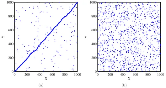
Such a correlation betweenX andY is called the cross-correlation and can be shown via plotting sample values ofX and Y jointly in a 2D-scatter plot. Figure 2.1 gives an example of showing the correlation with a 2D-scatter plot, where the cross-correlation in Figure 2.1(a) is clearer and stronger than that in Figure 2.1(b) since most joint sample values ofX andY in Figure 2.1(a) are distributed over a straight line. It is also possible to quantitatively measure the cross-correlation betweenX and Y via calculating their correlation coecient as
ρX,Y =E[(X−µX)(Y −µY)]
σXσY
2.2. Representations of Arrival Events 15
0 200 400 600 800 1000 0
200 400 600 800 1000
X
Y
(a)
0 200 400 600 800 1000 0
200 400 600 800 1000
X
Y
(b)
Figure 2.1: Example of the cross-correlation between two stochastic point processes, shown by their 2D-scatter plot.
The calculation of ρX,Y in Eq. 2.2 is called the Pearson correlation coecient.
The cross-correlation betweenX andY can also be checked by Spearman's approach. Spearman correlation coecient is dened as the Pearson correlation coecient ap-plied to the ranks of data instead of the data itself. The values of each variable are sorted: the lowest value with rank 1, the next lowest value with rank 2 and so on. Equal values are given an averaged rank, for example, if there are two equal values that are ranked 5 and 6, they are both given rank 5.5.
2.2
Representations of Arrival Events
In a system workload, an arrival process, which refers to either arrivals of jobs or of Bags-of-Tasks, can be described as a series of individual time events {tn}, where a
job or a Bag-of-Tasks arrives on each timeti. There exist dierent representations of
an arrival process [48] as illustrated in Figure 2.2. Firstly, as an interarrival process which is a sequence {In} with In = tn−tn−1. Secondly, as a count process which depends on a pre-selected time interval T and is obtained by dividing the time axis into equally spaced continuous intervals ofTto yield a sequence of counts{Cn}, where
Cn is the number of time events in thenth interval. Thirdly, as a rate process{Rn}
that is based on the count process, whereRn =Cn/T. We call each distinct value of
16 Chapter 2. Background Knowledge
(a)
(b)
(c)
Figure 2.2: An illustration of representing an arrival process (a) by an interarrival process (b) and a count or rate process (c) withT = 15.
Each representation has its own advantage and drawback [47]. Representing a point process with{Cn}or{Rn}causes a loss of information about the times between
arrival events within an intervalT. On the contrary,{In}keeps the whole information
and so can be used to recreate the original point process accurately. However, the direct correspondence between its index number and the absolute time is lost. This shortcoming of{In}is the advantage of {Cn} and{Rn}in contrast.
2.3
Definitions of Workload Features
run-2.3. Definitions of Workload Features 17
time and parallelism, where each attribute is represented as a point process. Hence, the term workload used in this thesis is a combination of three point processes: the arrival time process{An}, the runtime process{Rn}and the parallelism process
{Pn}, where a jobiin the workload is represented by the trippleAi,Ri andPi. The
term workload feature refers to the characteristics of the point processes forming the workload, which are described in the rest of this section.
2.3.1
Features of an Arrival Process
Three characteristics of arrival events are studied, namely long range dependence, periodicity and temporal burstiness.
0 24 48 72 96 120 144 −0.2
0 0.2 0.4 0.6 0.8 1
Lag
ACF
Figure 2.3: An illustration of long range dependence.
Long Range Dependence
A discrete-time second-order stationary processX(t)is said to be long range depen-dent (LRD) if its autocorrelation functionR(k)satises the condition
R(k)∼ck2H−2 ask→ ∞, (2.3)
18 Chapter 2. Background Knowledge
P∞
k=0R(k) =∞. Figure 2.3 gives an illustration of a LRD process shown by its ACF. LRD can be quantitatively measured by the Hurst parameter H which takes on values from 0.5 to 1. A value of 0.5 indicates the absence of LRD. The closer H is to 1, the greater the degree of LRD. For a deeper understanding, see [6, 19, 84].
Periodicity
In the context of parallel systems, the characteristic periodicity is observed because jobs are often submitted in cycles. The length of a cycle can be in the order of hours, days, months, years or any time length. The daily cycle is the most known and widely recognized cycle since it appears in all practical workloads [19, 116]. Parallel system workload cycles typically show a higher activity during the day and a lower activity during the night. However, details including cycle lengths may dier among dierent workloads.
Detecting the periodicity of a point process can be done via its autocorrelation function. An illustration of a process with periodicity is given in Figure 2.4. We can visually observe cycles in its ACF. The autocorrelation at lag 0 is 1 because the process is compared with itself, thus, the ACF results an exact match. Then when the lag increases, the autocorrelation quickly decays. As we can see, the ACF repeats every 24 lags since the process tends to match itself whenever the lag is an integral multiple of 24. For a deeper understanding, see [19].
0 24 48 72 96 120 144 −0.2
0 0.2 0.4 0.6 0.8 1
Lag
ACF
2.3. Definitions of Workload Features 19
Temporal Burstiness
In the context of system job trac, we refer to temporal burstiness as the tendency of job arrivals to occur in bursts, separated by long periods of no arrivals. Since there exists no generally accepted denition for temporal burstiness despite its prevalence [42], we nd that a denition that is closest to our work should be based on the concepts of burst and gap. A burst consists of job arrivals whose interarrival times are small while a gap refers to a large interarrival time. An illustration of our denition of temporal burstiness in job trac is given in Figure 2.5, where we show two job arrival processes with dierent degrees of temporal burstiness. Job arrivals 2 are more bursty than job arrivals 1 because they have tighter bursts and longer gaps. For the concept of temporal burstiness in this thesis, we use the coecient of variationCv of
interarrival times as a metric. If a job arrival process exhibits tight bursts and long gaps, it will result in a largeCv, indicating a large degree of temporal burstiness.
Figure 2.5: An illustration of temporal burstiness in two system job traffics.
2.3.2
Features of Runtime and Parallelism
Three characteristics are presented in this section, consisting of the temporal locality structure of a runtime process, spatial burstiness and the correlation between runtime and parallelism.
Temporal Locality
20 Chapter 2. Background Knowledge
consists of 4 jobs with runtimes R1 = {10,12,15,9}, the second BoT has R2 =
{3000,2800} and the third BoT contains R3 = {400,360,420}. These BoTs form a runtime process R = {10,12,15,9,3000,2800,400,360,420}. Assume we have an ecient approach (as is introduced later in Section 3.3.1) to classify R in such a way that similar runtimes are grouped to the same cluster1. Then we will have a series of cluster labels corresponding to R: L ={A, A, A, A, C, C, B, B, B}. We use Lto form a series of lengths of repetitions: LR={4,2,3}because the cluster labels A, C and B are repeated 4, 2 and 3 times, respectively. As such, we can see from L and LR that the common BoT behaviour in parallel workloads will lead to the phenomenon of repetitions in a runtime process. The term temporal locality refers to this phenomenon and the bigger the elements of LR, the larger the degree of temporal locality.
Spatial Burstiness
Spatial burstiness of a parallel workload refers to the non-uniformity of the distribu-tions of runtimes and parallelisms. This non-uniformity can be observed via drawing a 3D-histogram of the runtimes and the parallelisms. Figure 2.6 gives an example of spatial burstiness. Observing two 3D-histograms in the gure, we see that Workload2 has a low degree of spatial burstiness because of its relatively at 3D-histogram in Figure 2.6(b) while Workload1 in Figure 2.6(a) has a higher degree of spatial bursti-ness.
For a quantitative measure of spatial burstiness, we propose a new entropy-based approach to quantify it in a parallel workload. In information theory, entropy is common in measuring uniformity. The entropy of a random variableX is dened [90] as
H(X) =−
N
X
i=1
pi×logpi, (2.4)
where pi indicates the probability for event Xi to happen. In our work, we measure
spatial burstiness with a normalized entropy. It is known [33] that the entropy in Eq. (2.4) has a minimal value of 0 when for some j,pj= 1 andpi= 0,i6=j. It reaches
its maximal value oflogN when pi = 1/N,i= 1, . . . , N. As such,H(X)in general
will increase withN. Hence, the normalized entropy HN E of a random variableX,
dened as
HN E(X) = −
PN
i=1pi×logpi
logN , (2.5)
1The term “cluster” stems from the concept of “clustering”. Clustering is the assignment of a set
2.3. Definitions of Workload Features 21
will be bounded by 0 and 1. The disadvantage of quantifying spatial burstiness based on the normalized entropy is the dependency on the number of ranges N since it is necessary to divide the space axis into N ranges and calculate the probability for an event to happen on each range. If N changes, the probabilities will also change. This leads to dierent values of the normalized entropy and thus gives an instable measure2. However, with parallel workloads, we nd an ecient method to eliminate this dependency by deningpi in Eq. (2.5) exibly. For a workloadW, we calculate
pi as pi = T Ri/T R, where T Ri is the total runtime of all jobs in W that request
i processors and T R is the total runtime of all jobs in W. As such, the value of N is equal to the maximal number of processors that a job may request in W, and therefore the measure is stable. Furthermore, since the entropy is normalized, this metric only ranges from 0 to 1. The closer the metric is to 0, the stronger the spatial burstiness.
(a) (b)
Figure 2.6: Example of spatial burstiness of two workloads by using 3D-histograms to show the distribution of jobs according to their runtimes and parallelisms.
Correlation between Runtime and Parallelism
The correlation between runtime and parallelism can be checked simply by calculating their correlation coecient. The value of a correlation coecient ranges from−1 to
2Wang et al. in [110] used the entropy function in Eq. (2.4) to measure the temporal-spatial
22 Chapter 2. Background Knowledge
+1. A negative value indicates that smaller runtimes tend to be associated with larger numbers of processors. This means large applications often use more processors to reduce their runtimes based on the implicit assumption that their total amount of work remains the same. Vice versa, a positive value shows the tendency of the association between smaller runtimes and smaller numbers of processors. If a workload exhibits a positive correlation, the implicit assumption above is no longer correct. It means that large applications often run longer with more processors.
As presented in Section 2.1.3, the correlation coecient between two point pro-cesses can be calculated by using Pearson's or Spearman's approach. However, Pear-son's approach is not strong enough to capture correlation since it works well under many assumptions and one is that the two processes follow normal distributions, but this is not the case for real world data such as job runtimes and numbers of processors. Spearman's approach, which uses the data ranks instead of the data itself to calculate the correlation coecient, is more suitable to examine correlation, in particular when we want to know if smaller runtimes are associated with smaller or larger numbers of processors. Therefore, Spearman's approach is used in this research.
2.3.3
The Bag-of-Tasks Behaviour
We consider a parallel workload W as an ordered set of N jobs: W = {Ji|i =
1, . . . , N andAT(Ji)≤AT(Jj) ifi < j}, whereAT(·)denotes the arrival time. Since
there is no general denition of the Bag-of-Tasks (BoT) behaviour for parallel work-loads, we dene a BoT with a time parameter∆as a maximal contiguous subsequence B ofW such that
1. For any two successive jobsJi,Ji+1 inB, we haveAT(Ji+1)≤AT(Ji) + ∆.
2. All jobs in B have the same values with respect to user name, group name, queue name, job name, estimated runtime and number of processors.
Similar to a job, a BoT also has its own attributes which are dened as follows:
1. The arrival time of a BoT is the minimal arrival time of jobs within the BoT. 2. The submission duration of a BoT is the dierence between the maximal and
the minimal arrival times of jobs within the BoT. 3. The size of a BoT is the number of jobs in the BoT.
2.4. Summary 23
the parallelism and the estimate of a BoT as the average of the runtimes of all jobs, the requested number of processors and the user estimated runtime of any job in the BoT, respectively. We have chosen this denition because it can help to simplify modeling research. For example, a model can easily create all jobs in a BoT after determining the size, the runtime, the parallelism and the estimate of the BoT because we know the number of jobs in the BoT, the runtimes, the requested numbers of processors and the user estimated runtimes of the jobs via the size, the runtime, the parallelism and the estimate of the BoT. The remainder that the model needs to handle is to decide the interarrival times of the jobs.
2.4
Summary
Chapter 3
Statistical Analysis
Any research of modeling and performance evaluation that centers around workloads should begin with a study of workload characterisation. Therefore, this chapter fo-cuses on a statistical analysis of parallel system workloads that will help to enrich the understandings of a system and the workload running on it. In addition, the analysis is also applied to grid traces to show that some features of parallel workloads can be observed on grid data and, thus, it is possible to apply research results in later chap-ters to grids. In particular, we emphasize the Bag-of-Tasks (BoT) behaviour because it has become more common in scheduling and modeling research [2, 39, 71, 109, 112]. According to the BoT denition, a BoT can consist of only one job. In our analysis, we only take into account BoTs that contain at least 2 jobs (so-called real BoTs), except for characterising BoT arrivals. BoTs with a single job (so-called unreal BoTs) are not excluded in this case because in practice, real and unreal BoTs arrive in a mixed way. Hence, excluding unreal BoTs in an arrival process causes a loss of information about interarrival times since arrival events of unreal BoTs are discarded.
The chapter rstly introduces the data used in the analysis and provides infor-mation about where the data are collected and how they are pre-processed so that research results presented in this thesis can be reproduced. After that, the workload features introduced in Chapter 2 are analyzed statistically. Finally, we discuss their important roles in clusters, grids and clouds to indicate that it is essential to take them into modeling and evaluate their performance impacts on parallel systems.
3.1
Workload Data under Study
26 Chapter 3. Statistical Analysis
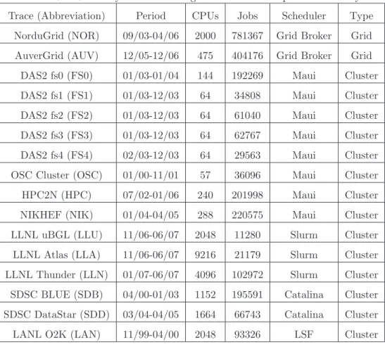
illustrate that part of our work can be applied successfully for grid jobs. Note that we remove from NorduGrid the rst 3 jobs due to the abnormal long interarrival time (∼5 months) between the third and fourth jobs. The parallel and grid traces, except for NIKHEF, can be obtained from the Parallel Workloads Archive [80] and the Grid Workloads Archive [31], respectively. Note that, there are two versions for every logged trace on the Parallel Workloads Archive. The original version is the collected data while the cleaned version removes a number of jobs from the original version because the original data often includes problematic and unrepresentative data, such as signicant automated administrative activity or large-scale urries of activity by single users [80]. In our study, we use the cleaned version for all parallel workloads as recommended on the Parallel Workloads Archive, which is based on [23, 106]. The cluster NIKHEF is located at the High Energy Physics institute in the Netherlands, which participates in the LCG grid [44]. The names of the other traces are equal to those mentioned on the two websites [31, 80] so that their full details can be retrieved easily.
Table 3.1: Summary of cluster and grid data used in experimental study.
Trace (Abbreviation) Period CPUs Jobs Scheduler Type
NorduGrid (NOR) 09/03-04/06 2000 781367 Grid Broker Grid
AuverGrid (AUV) 12/05-12/06 475 404176 Grid Broker Grid
DAS2 fs0 (FS0) 01/03-01/04 144 192269 Maui Cluster
DAS2 fs1 (FS1) 01/03-12/03 64 34808 Maui Cluster
DAS2 fs2 (FS2) 01/03-12/03 64 61040 Maui Cluster
DAS2 fs3 (FS3) 01/03-12/03 64 62767 Maui Cluster
DAS2 fs4 (FS4) 02/03-12/03 64 29563 Maui Cluster
OSC Cluster (OSC) 01/00-11/01 57 36096 Maui Cluster
HPC2N (HPC) 07/02-01/06 240 201998 Maui Cluster
NIKHEF (NIK) 01/04-04/05 288 220575 Maui Cluster
LLNL uBGL (LLU) 11/06-06/07 2048 11280 Slurm Cluster
LLNL Atlas (LLA) 11/06-06/07 9216 21179 Slurm Cluster
LLNL Thunder (LLN) 01/07-06/07 4096 102972 Slurm Cluster
SDSC BLUE (SDB) 04/00-01/03 1152 195591 Catalina Cluster
SDSC DataStar (SDD) 03/04-04/05 1664 66743 Catalina Cluster
3.2. Job Arrival Analysis 27
3.2
Job Arrival Analysis
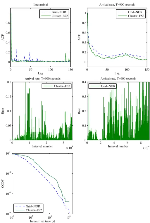
We draw in Figure 3.1 dierent statistics of job arrivals from a grid trace and a cluster trace. As we can observe from the autocorrelation functions (ACFs), if represented as an interarrival process, job arrivals do not exhibit a correlation structure. However, if represented by a rate process, job arrivals do exhibit the long range dependence (LRD) feature clearly. This is consistent with the study in [46], which concludes that LRD of system job arrivals should be reliably revealed in count/rate-based measures. This is the reason why we use the rate process representation for LRD of job arrivals.
We quantitatively measure the degree of LRD in the real traces by estimating the Hurst parameter and show the results in Table 3.2. We select three estimators, namely Aggregate Variance, R/S Statistic and Periodogram [101], and calculate the mean and the standard deviation of their estimates. We can see from Table 3.2 that LRD is present strongly in real job arrivals since the estimated results are much larger than 0.5.
Table 3.2: The Hurst parameter of rate processes (T=900 seconds).
Trace Hurst parameter
NOR 0.86±0.07
AUV 0.91±0.06
FS2 0.77±0.10
FS3 0.84±0.09
HPC 0.70±0.09
LAN 0.80±0.03
LLN 0.69±0.17
NIK 0.70±0.08
With respect to temporal burstiness, we argue that it has to be exhibited in real job arrivals due to the occurrence of Bags-of-Tasks and idle periods during nights, weekends, holidays, etc. when users often submit fewer jobs. As we can see from Figure 3.1, the interarrival time distributions of both grid and cluster traces are heavy-tailed and so the temporal burstiness is observed. We measure the temporal burstiness degree in real job arrivals in Table 3.3 by applying the metric coecient of variation Cv to interarrival times. As a distribution with a Cv smaller than 1 is
28 Chapter 3. Statistical Analysis
0 50 100 150
0 0.2 0.4 0.6 0.8 1 Lag ACF Interarrival Grid−NOR Cluster−FS2
0 50 100 150
0 0.2 0.4 0.6 0.8 1 Lag ACF
Arrival rate, T=900 seconds
Grid−NOR Cluster−FS2
0 1 2 3
x 104 0
0.05 0.1 0.15 0.2
Arrival rate, T=900 seconds
Interval number
Rate
Cluster−FS2
0 2 4 6 8
x 104 0 0.1 0.2 0.3 0.4 Interval number Rate
Arrival rate, T=900 seconds
Grid−NOR
100 102 104 106
10−6 10−4 10−2 100
Interarrival time (s)
CCDF
Grid−NOR Cluster−FS2
3.3. Runtime and Parallelism 29
Table 3.3: Temporal burstiness of cluster/grid job arrivals, expressed by the coeffi-cient of variation.
Trace Coefficient of variation
NOR 33.14
AUV 5.65
FS2 13.88
FS3 17.92
HPC 5.70
LAN 17.70
LLN 10.00
NIK 18.56
3.3
Runtime and Parallelism
This section shows a common presence of the correlation between runtime and paral-lelism as well as the features temporal locality and spatial burstiness in a large number of real traces. According to the denition of temporal locality, we need an ecient approach to classify a job runtime process in such a way that similar runtimes are grouped to the same cluster. Therefore, we start this section by introducing such a classication framework and continue by examining the three characteristics in real workloads.
3.3.1
Runtime Classification
30 Chapter 3. Statistical Analysis
3.3.2
Examination of Correlation
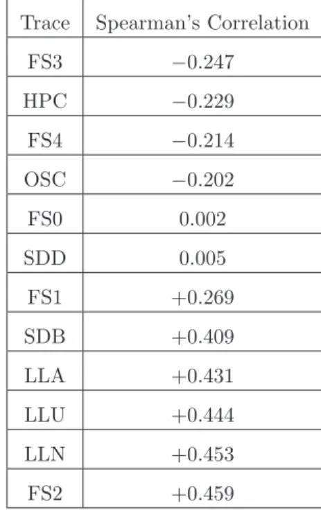
We calculate the correlation between runtime and number of processors in real work-loads and show the results in Table 3.4. As one can see, the correlation feature commonly exists in real world data because 10 of 12 traces exhibit correlations with 4 negative and 6 positive, while only 2 traces show that runtime and parallelism are not correlated with correlations around 0. A notable point is that negative correla-tions concentrate around the value of−0.2 and for positive correlations around+0.4. Therefore, when we study the performance issues of locality, we will focus on three realistic degrees of correlation, namely−0.2,0and+0.4, as is shown later in Chapter 7.
Table 3.4: The feature correlation between runtime and parallelism of real parallel workloads, expressed by applying Spearman’s approach.
Trace Spearman’s Correlation
FS3 −0.247
HPC −0.229
FS4 −0.214
OSC −0.202
FS0 0.002
SDD 0.005
FS1 +0.269
SDB +0.409
LLA +0.431
LLU +0.444
LLN +0.453
FS2 +0.459
3.3.3
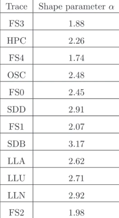
Examination of Temporal Locality
3.3. Runtime and Parallelism 31
P(x)∼ 1
xα withα >0, (3.1)
where α is a shape parameter. As from Eq. (3.1), the larger the value of α, the exponentially smaller the probability for the occurence of a big length of repetitions and thus the smaller the degree of temporal locality.
Table 3.5: The feature temporal locality of real parallel workloads, expressed by estimating the shape parameterαof a Zipf distribution.
Trace Shape parameterα
FS3 1.88
HPC 2.26
FS4 1.74
OSC 2.48
FS0 2.45
SDD 2.91
FS1 2.07
SDB 3.17
LLA 2.62
LLU 2.71
LLN 2.92
FS2 1.98
By applying the Model-Based Clustering framework on real traces, we obtain series of cluster labels and based on that, we calculate series of lengths of repetitions. We present the temporal locality feature of real traces in Figure 3.2 by drawing the log-log histograms of lengths of repetitions. Visually, the histogram of a Zipf distribution will show a straight line with a negative slope using log-log axes. However, the tail of the Zipf distribution is hard to characterise because there are many big sizes that each appears only a few times, and thus it shows more diversity at the tail. As observed from Figure 3.2, the lengths of repetitions in the real world data are tted well to Zipf distributions and thus the temporal locality feature of the real traces can be determined by estimating the shape parameter α of the Zipf distributions1.
1Note, we only use the shape parameterαof a Zipf distribution to determine the phenomenon of
32 Chapter 3. Statistical Analysis
100 103
100 105
Length of repetitions
Number of occurences
FS0
100 103
100 105
Length of repetitions
Number of occurences
HPC
100 103
100 105
Length of repetitions
Number of occurences
LLN
100 103
100 105
Length of repetitions
Number of occurences
OSC
100 103
100 104
Length of repetitions
Number of occurences
FS4
100 103
100 106
Length of repetitions
Number of occurences
SDB
3.4. Basic Analysis of Bag-of-Tasks 33
The estimated results ofαare shown in Table 3.5. It can be seen that the temporal locality property exists commonly in real traces and its degree varies among the real workloads. Therefore, we believe that temporal locality deserves to be taken into account to evaluate its eect on scheduling.
3.3.4
Examination of Spatial Burstiness
To characterise spatial burstiness in real parallel workloads, we apply the approach of using normalized entropy proposed in Section 2.3.2 and show the results in Table 3.6. An interesting observation from the results is that the feature spatial burstiness exists clearly in real data because the results are closer to 0 than 1. This observation suggests that this property deserves to receive more attention in the literature. The study on the impact of this characteristic on scheduling should be emphasized so that correct workloads are used in evaluating scheduling algorithms.
Table 3.6: The normalized entropy of spatial burstiness.
FS2 FS3 HPC LAN LLN
0.447 0.126 0.305 0.317 0.330
3.4
Basic Analysis of Bag-of-Tasks
This section analyzes many basic features of the Bag-of-Tasks behaviour. As noticed in the BoT denition, forming a BoT depends on the parameter∆. Therefore, in order to determine a suitable value for this parameter, we dene the set S of a workload W as including all interarrival times (IATs) between any two successive jobsJi,Ji+1 in W such thatJi andJi+1 have the same values for user name, group name, queue name, job name, estimated runtime and number of processors. According to the BoT denition,JiandJi+1can belong to the same BoT. However, ifJi terminates before
Ji+1 arrives, we exclude their IAT fromS because when users know the result ofJi,
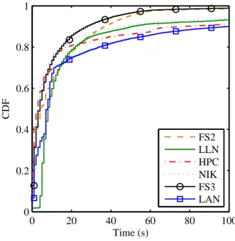
they may adjustJi+1and therefore,Ji andJi+1 should not belong to the same BoT. In Figure 3.3, we draw the cumulative distribution functions (CDFs) of all IATs for all six parallel traces. From the gure we see that most IATs do not exceed 100 seconds. Therefore, we select∆ = 100seconds in our study because larger values do not much increase a BoT size but reduce the meaning of a BoT.
34 Chapter 3. Statistical Analysis
0 20 40 60 80 100 0
0.2 0.4 0.6 0.8 1
CDF
Time (s)
FS2 LLN HPC NIK FS3 LAN
Figure 3.3: The cumulative distribution functions of IATs in six parallel traces.
Table 3.7: Fraction of jobs submitted as part of BoTs.
FS2 FS3 HPC LAN LLN NIK
60% 89% 65% 34% 40% 83%
as part of BoTs, as is shown in Table 3.7. Hence, we conclude that BoTs should be incorporated into a workload model.
Another issue of BoTs that could be important for modeling is the runtimes of jobs within a BoT. We have reason to believe that the runtimes will be similar because the jobs have the same values for other attributes such as user and group names, etc. To check this, we compute the average coecient of variationCv of the runtimes in the
BoTs. As a distribution with aCv <1is considered to have low variance, runtimes
in a BoT exhibit low variance since the average Cv is smaller than 1 and closer to 0
as shown in Table 3.8. Therefore, we conclude that jobs within a BoT have similar runtimes.
Table 3.8: The average coefficient of variation of the runtimes of the jobs in a BoT.
FS2 FS3 HPC LAN LLN NIK
3.5. BoT Arrival Analysis 35
The question of the length of the submission duration of a BoT is also interesting. We dene the submission duration of a BoT as the dierence between the maximal and the minimal arrival times of jobs within the BoT. To determine how big in time a BoT is, we draw the cumulative distribution functions of these durations of the real data. As we can see from Figure 3.4, for all three workloads, almost 100% of the BoT submission durations are smaller than 15 minutes.
100 101 102 103 104 0
0.2 0.4 0.6 0.8 1
CDF
Time (s)
FS0 HPC LLN
Figure 3.4: The cumulative distribution functions of BoT submission durations in the real workloads.
The last BoT-related issue that could be taken into account in a workload model is the distribution of BoT sizes. As we indicate in Section 3.3.3, runtimes of parallel workloads tend to be similarly repetitive and Feitelson [18] shows that runlengths2 can be tted by a Zipf distribution. Since job runtimes of a BoT are similar, it is possible that a Zipf distribution can also be applied for BoT sizes. This is indeed conrmed in Figure 3.5.
3.5
BoT Arrival Analysis
We introduce in Section 2.2 that an arrival process can be represented by either an interarrival process or a count/rate process. In this section, we start with the
36 Chapter 3. Statistical Analysis
100 101 102
100 101 102 103 104
BoT size / Runlength
Number of occurences
FS3
Runlength BoT size
100 101 102
100 101 102 103 104 105
BoT size / Runlength
Number of occurences
LAN
Runlength BoT size
Figure 3.5: Log-log histograms of BoT sizes (including sizes equal to 1) and run-lengths in real traces.
analysis of BoT arrivals in terms of their interarrival times to characterise the temporal burstiness. Then, we represent BoT arrivals by a rate process to characterise long range dependence and periodicity features.
3.5.1
Interarrival Times and Temporal Burstiness
3.5. BoT Arrival Analysis 37
is larger than that of the Weibull distribution, KS statistics of both distributions are close to 0 and therefore both distributions can be tted well to the data as shown in Figure 3.6(b). From this result, we argue that the Generalized Pareto distribution should be used for modeling BoT arrivals.
Table 3.9: Parameters of distributions estimated during the fitting process.
a, b, θ, µ, σindicate shape, scale, threshold, mean and standard deviation, respectively.
Dist. GP(a, b, θ) Wbl(a, b) LogN(µ, σ) Gam(a, b) Exp(µ)
FS0 1.12 67.53 0 0.51 170.36 4.02 3.13 0.35 1100 383.71
FS2 0.81 165.99 0 0.38 252.31 3.73 5.52 0.22 4887 1085.29
FS3 1.26 132.94 0 0.39 374.64 4.48 4.09 0.21 12826 2723.14
HPC 1.26 172.2 0 0.47 475.43 4.91 3.46 0.31 3874 1213.38
LLN 0.96 40.23 0 0.57 91.98 3.6 2.32 0.41 438 180.02
NIK 1.22 109.27 0 0.29 166.28 2.47 7.23 0.19 3101 589.2
Table 3.10: KS statistics obtained from KS tests.
Dist. GP Wbl LogN Gam Exp
FS0 0.059 0.098 0.182 0.118 0.348
FS2 0.098 0.237 0.323 0.212 0.478
FS3 0.063 0.106 0.192 0.237 0.604
HPC 0.074 0.054 0.139 0.103 0.355
LLN 0.063 0.127 0.143 0.137 0.322
NIK 0.152 0.212 0.284 0.197 0.286
A good t of the Generalized Pareto distribution to BoT interarrival times in real data implies that BoT arrivals are bursty. We quantitatively measure the temporal burstiness feature using the metric coecient of variationCv. This metric is equal to
0 if arrivals are not bursty. The larger this metric is, the burstier the arrivals are. The results in Table 3.11 show that BoTs are submitted to parallel systems in a bursty way.
3.5.2
Long Range Dependence and Periodicity
38 Chapter 3. Statistical Analysis
100 101 102 103 104 105 0 0.2 0.4 0.6 0.8 1 CDF Time (s) FS0 FS2 FS3 HPC LLN NIK (a)
100 101 102 103 104 105 0 0.2 0.4 0.6 0.8 1 CDF Time (s) HPC GP WBL LOGN GAM EXP (b)
Figure 3.6: Cumulative distribution functions of BoT interarrival times of real work-loads (a) and of HPC2N and fitted distributions (b).
Table 3.11: Temporal burstiness of BoT arrivals expressed as the metric coefficient of variation.
FS0 FS2 FS3 HPC LLN NIK
7.7 9.6 7.7 3.8 8.3 9.9
our study, we characterise both BoT and job arrivals to achieve a comparison of how dierent they arrive on parallel systems. We select a time scale equal to 15 minutes for converting an arrival process to a rate process because we have shown in Section 3.4 that almost 100% of the BoT submission durations are smaller than 15 minutes.
3.5. BoT Arrival Analysis 39
0 500 1000 1500
0 0.2 0.4 0.6 0.8 1 Lag ACF FS0 Job BoT
0 500 1000 1500
0 0.2 0.4 0.6 0.8 1 Lag ACF HPC Job BoT
0 500 1000 1500
0 0.2 0.4 0.6 0.8 1 Lag ACF FS2 Job BoT
0 500 1000 1500
0 0.2 0.4 0.6 0.8 1 Lag ACF LLN Job BoT
0 500 1000 1500
0 0.2 0.4 0.6 0.8 1 Lag ACF FS3 Job BoT
0 500 1000 1500
0 0.2 0.4 0.6 0.8 1 Lag ACF NIK Job BoT
40 Chapter 3. Statistical Analysis
but no periodicity while job arrivals have a smaller degree of LRD and exhibit a weak daily cycle. Finally for FS0, job arrivals show a larger dependence and a longer cycle (weekly versus daily) comparing with BoT arrivals. As such, it is clear that job trac in parallel systems is a complex problem. BoT arrivals can have similar structures as job arrivals, but they can also be completely contrary. Therefore, we believe that trac models in parallel systems should take care of this problem and more research on modeling job trac should be done to provide models that are as realistic as possible.
Table 3.12: LRD of job and BoT arrivals expressed by estimating the Hurst param-eterH.
FS0 FS2 FS3 HPC LLN NIK
Job 0.85 0.79 0.74 0.67 0.78 0.69
BoT 0.76 0.86 0.73 0.81 0.79 0.68
3.6
BoT Size, Runtime, Parallelism and Estimate
In this section, we focus our analysis on four attributes of BoTs, namely size, run-time, parallelism and estimate. The characterisation will concentrate on examining the autocorrelations and the cross-correlations between these BoT attributes. Figure 3.8 shows that BoT runtimes can exhibit weak to strong autocorrelations. The au-tocorrelation in the sequence of BoT runtimes occurs because users tend to submit the same applications over and over again. This behaviour of users also causes the autocorrelation of job runtimes. However, calculating the autocorrelation in the se-quence of job runtimes will be aected by the repetitions of similar jobs in the same BoT. Consequently, it yields larger autocorrelations and job runtimes become more sensitive with the autocorrelation function at short lags. Therefore, we argue that the autocorrelation should be calculated based on BoT runtimes instead of job runtimes. With respect to the attribute BoT size, we investigate and show in Table 3.13 its statistics consisting of the mean and the maximum size. A noticeable point is that BoT sizes of 4 (FS0, FS2, HPC and NIK) out of 6 traces have similar means. Furthermore, the maximum size of a BoT is rather large and can be up to thousands of jobs. Parallel systems can undergo durations of severe congestion when such a large BoT occurs. Hence, we claim that realistic BoT workloads used in scheduling evaluation should contain large BoTs with hundreds to thousands of jobs for a reliable evaluation result.
3.6. BoT Size, Runtime, Parallelism and Estimate 41
0 50 100 150 200 −0.1
0 0.2 0.4 0.6 0.8 1
Lag
ACF
FS0 HPC LLN NIK
Figure 3.8: Autocorrelation functions of BoT runtimes.
Table 3.13: Statistics of BoT sizes.
FS0 FS2 FS3 HPC LLN NIK
Mean 7 8 14 7 5 8
Max 1263 558 3675 2418 169 1201
expected that BoT runtimes would decrease if BoT sizes increase. This should give negative correlations, because we think that users would divide their applications into several smaller jobs by increasing their BoTs. However, results in Table 3.14 tell us that our expectation seems to be correct only for NIK. For FS2 and LLN, the correlations are also negative but rather weak, and in contrast FS0, FS3 and HPC show positive correlations. This means that if users increase their BoT sizes, jobs tend to run longer and this will harm the performance of parallel systems. Therefore, we believe that modeling and scheduling studies should take care for this realistic situation.
Table 3.14: Correlation between BoT sizes and BoT runtimes.
FS0 FS2 FS3 HPC LLN NIK
42 Chapter 3. Statistical Analysis
Our next expectation is that BoT parallelisms will decrease if BoT sizes increase. Results of calculating the correlation between the two attributes, shown in Table 3.15, conrm our expectation in case of FS2, FS3 and HPC since their correlations are negative (the other traces also produce negative correlations but rather weak). We predict this result because we believe that users should reduce the numbers of requested processors when they increase their BoT sizes. Otherwise, there could be not enough free processors to be allocated to their jobs.
Table 3.15: Correlation between BoT sizes and BoT parallelisms.
FS0 FS2 FS3 HPC LLN NIK
-0.032 -0.198 -0.310 -0.150 -0.091 -0.014
Finally, we calculate the correlation between the size and the estimate and show results in Table 3.163. As we see, the correlation is negative in case of FS2, FS3 and NIK. This means that users of these systems tend to take initiative to reduce the amount of time they request for their jobs when they increase the size of BoTs, possibly because they do not want schedulers to let their jobs wait long in waiting queues. However, users of the HPC system seem unconcerned about the longer times their jobs have to wait for execution because they tend to increase the estimate together with the size of their BoTs, shown by a positive correlation. To further our understanding of why HPC users tolerate the longer wait times, we calculate the occupation time and the estimated occupation time of BoTs4. Table 3.17 shows how much users utilize their estimates. Since HPC has the best utilization, HPC users seem to estimate their jobs better than users of other systems. Therefore, if HPC users decrease their estimates they may have the risk of underestimation, which can kill their jobs. To guarantee a successful execution for their jobs, they must tolerate longer wait times.
Table 3.16: Correlation between BoT sizes and BoT estimates.
FS0 FS2 FS3 HPC LLN NIK
-0.033 -0.244 -0.236 0.175 - -0.145
3Since 65% jobs of LLN do not have the information about their user estimates, we decide to skip
it when we analyze the BoT estimate.
4We define the occupation time of a job as the total time that it occupies processors, calculated
![Figure 1.1: The growth of parallel systems in terms of number of processors. Data are obtained from the TOP500 Supercomputing Sites [103].](https://thumb-us.123doks.com/thumbv2/123dok_us/8321201.2205602/13.723.101.623.326.610/figure-growth-parallel-systems-number-processors-obtained-supercomputing.webp)