B. Giammarinaro
UMR 7190, Institut Jean Le Rond d’Alembert, Sorbonne Universites, UPMC Univ Paris 06, Paris F-75005, France e-mail: [email protected]
F. Coulouvrat
CNRS, UMR 7190, Institut Jean Le Rond d’Alembert, Paris F-75005, France e-mail: [email protected]
G. Pinton
Joint Department of Biomedical Engineering, University of North Carolina at Chapel Hill and North Carolina State University, Chapel Hill, NC 27599 e-mail: [email protected]
Numerical Simulation
of Focused Shock Shear
Waves in Soft Solids and a
Two-Dimensional Nonlinear
Homogeneous Model of
the Brain
Shear waves that propagate in soft solids, such as the brain, are strongly nonlinear and can develop into shock waves in less than one wavelength. We hypothesize that these shear shock waves could be responsible for certain types of traumatic brain injuries (TBI) and that the spherical geometry of the skull bone could focus shear waves deep in the brain, generating diffuse axonal injuries. Theoretical models and numerical methods that describe nonlinear polarized shear waves in soft solids such as the brain are pre-sented. They include the cubic nonlinearities that are characteristic of soft solids and the specific types of nonclassical attenuation and dispersion observed in soft tissues and the brain. The numerical methods are validated with analytical solutions, where possible, and with self-similar scaling laws where no known solutions exist. Initial conditions based on a human head X-ray microtomography (CT) were used to simulate focused shear shock waves in the brain. Three regimes are investigated with shock wave forma-tion distances of 2:54 m;0:018 m, and 0:0064 m. We demonstrate that under realistic loading scenarios, with nonlinear properties consistent with measurements in the brain, and when the shock wave propagation distance and focal distance coincide, nonlinear propagation can easily overcome attenuation to generate shear shocks deep inside the brain. Due to these effects, the accelerations in the focal are larger by a factor of 15 com-pared to acceleration at the skull surface. These results suggest that shock wave focusing could be responsible for diffuse axonal injuries.[DOI: 10.1115/1.4032643]
1
Introduction
Shear waves in soft solids have nonlinear properties that are 4 orders of magnitude larger than in classical solids [1]. Conse-quently, shear waves can transition from a smooth to a shocked profile in less than one wavelength [2]. This extremely nonlinear behavior is largely due to the slow shear wave speed in soft solids, which is approximately 2 m=s [3] compared to 1540 m=s [4] for a compressional wave.
We hypothesize that these shear shock waves could be respon-sible for certain types of TBI and that the spherical geometry of the skull bone could focus shear waves, generating shocks. The sharp gradients occurring at shear shock wave front could stretch and damage neurons generating some lesions. This mechanism could be responsible for diffuse axonal injuries which occur deep in the brain, far from the impact surface, and appear as focal lesions.
Compared to acoustic shocks, which have been well studied in the context of TBI, very little is known about shear waves because until recently they were difficult to measure at depth in solids. Shear shock waves were observed for the first time in tissue-mimicking soft solids [1] in 2003, when the technology to obtain high frame-rate ultrasound imaging was developed [5]. Following this observation, a model for incompressible media was developed [6,7] leading to equations that describe nonlinear propagation of
plane shear waves for different polarizations in soft solids [8]. The approximation of incompressible media was investigated by Wochner et al. in 2008 [9]. The same authors extended the plane wave model by including diffraction in the paraxial approxi-mation. For a transverse polarization, the model reduces to an equation similar to the well-known Khokhlov–Zabolotskaya– Kuznetsov [10] in acoustics but with a cubic nonlinear term instead of a quadratic one. This leads to the nonlinear generation of odd harmonics (f0, 3f0;5f0,.) [11] and shock waves, which can be used to measure the nonlinear elastic parameters [12,13]. Non-linear Mach reflection of shear shock waves has also been studied theoretically and numerically [14]. Hence, there are strong simi-larities between shear shock waves and classical pressure shock waves.
Magnetic resonance elastography (MRE) has been used to investigate linear shear wave propagation in the brain [15,16]. By assuming a single frequency or narrowband input, the shear wave can be sampled with sub-Nyquist techniques at frame rates below the excitation frequency. Restricting the frequency content to a narrowband range that is known a priori allows the aliased signal to be unwrapped to the correct frequency. Then, by assuming lin-ear propagation, the Helmholtz inversion method can be used to determine the linear elastic properties of the brain [15]. MRE has been successful at probing the linear mechanics of the brain, espe-cially in in vivo studies. However, two principal limitations render it unsuitable for investigation of the nonlinear shear waves pro-posed here. First, shock waves are inherently broadband, so that sub-Nyquist sampling techniques cannot be used. Second, Manuscript received July 31, 2015; final manuscript received January 18, 2016;
inversion of linear wave models cannot be used since the propaga-tion is nonlinear. MRE tagging has pushed the achievable imaging frame rates up to a nominal maximum of 100 images/s [17]. The shock waves described here have harmonics that extend beyond 1100 Hz, which places them beyond the current sampling rates achievable with MRE.
Ultrasound scanners can generate imaging frame rates in excess of 10,000 images/s [1,5]. Algorithms that are tuned to measure motion from the raw radio frequency signals have a precision that can be better than 1lm [18,19]. Adaptive correlation based motion tracking has been used to generate quantitative movies of planar shear shock waves at this high precision and high frame-rates [20].
However, the focusing of shear shock waves has never been investigated to the best of our knowledge, while an extensive liter-ature is devoted to compression shock focusing in the context of focused beams used in medical applications [21,22] or of sonic booms [23,24]. Due to wave speed differences, the time scales associated with shear shock waves are much longer than acousti-cal shocks. The objective of the present study is to numeriacousti-cally investigate the focusing of shock shear waves.
Numerical methods used for the biomechanical models of the head are dominated by finite elements (FE) because they can accurately and easily model detailed anatomical structure of the skull and brain in conjunction with complex mechanical models [25]. With respect to shear deformations, the first FE models assumed linear elasticity [26,27]. More recent models used linear viscoelasticity combined with large deformation [28–30]. Nonlin-ear neo-Hookean constitutive laws have been introduced for the deviatoric part [31,32] with no other parameter than the linear Young modulus. Mendis [33] used a hyperelastic Mooney–Rivlin with two linear parameters, while Brands et al. [34] extended this model with two additional nonlinear parameters. In the present study, we consider exclusively the shear component of elastic deformation and we use the fully nonlinear incompressible elastic model of Hamilton et al. [6], in which nonlinear effects combine into a single measurable nonlinear parameter [13]. Unlike FE simulations, here the propagation medium is assumed to be homogeneous. Furthermore, the simulations presented here are in two dimensions and a perfect transfer from head motion to brain tissue is assumed. However, this is the first simulation of two-dimensional shear shock wave propagation in the brain.
The first part of this paper presents the theoretical model and numerical methods that describe nonlinear polarized shear waves in soft solids, such as the brain. This model and numerical solution include the cubic nonlinearities that are characteristic of soft solids and the specific types of nonclassical attenuation and dispersion observed in soft tissues. In this case, shear shock waves can be modeled by a parabolic equation with cubic nonlinearities. Attenuation in soft tissues is described by a semi-empirical law in the frequency domain. The model is solved numerically with a quasi-second order scheme based on a Strang splitting method. Diffraction is solved with a Crank–Nicolson finite different scheme and nonlinearities by a modified MacDonald–Ambrosiano shock capturing scheme. In the second part, several numerical tests are used to validate this scheme. In particular, Guiraud’s self-similarity law was used as a demanding numerical test for two-dimensional shock waves. This provides the strongest avail-able numerical validation since there are no known analytical solutions of the full equations. The third part presents an idealized case of nonlinear shear wave focusing with initial conditions that are characteristic of TBIs. This allows us to numerically test the hypothesis that some TBIs could be caused by focusing the shear waves to generate shocks. In particular, an X-ray CT of a human skull is used as an initial condition surface that sends shear waves into the brain.
A two-dimensional head configuration for blunt impacts was then investigated. Skull geometry was retrieved from CT images. Mechanical brain properties were found in literature, except the nonlinear parameter which is unknown. Simulations were
therefore performed with a value obtained from tissue-mimicking phantom gels.
We demonstrate that under realistic loading scenarios and when the shock wave propagation distance and focal distance coincide, nonlinear propagation can easily overcome attenuation to generate shear shocks deep inside the brain. These results sug-gest that shock wave focusing could be responsible for diffuse axonal injuries.
2
Theoretical and Numerical Model
Soft solids such as the white or gray brain matter or gelatin-based phantoms can be considered, to the first order, as incom-pressible since there is a 3 order of magnitude difference between the shear cTand compressioncLwave propagation speeds. This
corresponds, respectively, to shear moduli on the order of a few kilopascals and to bulk moduli on the order of a few gigapascals, i.e., a difference of 6 orders of magnitude. By assuming a per-fectly incompressible behavior, the energy density, E, based on Landau and Lifshitz’ choice of invariants [6,35], can be written as
E¼lI2þA 3I3þDI
2
2 (1)
Here,I2¼trðS2Þ;I3¼trðS3Þ, andSis the fully nonlinear strain tensor related to the displacement fielduby
Sij¼ 1 2
@ui
@xj þ@uj
@xi þ@uk
@xi
@uk
@xj
(2)
The shear modulus isl¼qc2
T,q is the medium density, and A and D are, respectively, the third- and fourth-order elastic constants.
In the case of a perfect linear polarization u3ðx1;x2;tÞ, the elastodynamic equations reduce to a nonlinear scalar wave equa-tion [14]
q@
2u3
@t2 ¼l
@2u3
@x2 2
þ@ 2u3
@x2 1
!
þ lþA 2þD
@
@x2
@u3
@xm
@u3
@xm
@u3 @x2 þ @ @x1 @u3
@xm
@u3
@xm
@u3
@x1
(3)
with a sum on the indexm¼1 and 2. This equation can be further simplified by using the paraxial approximation [9]. Then, the wave propagates mainly in theX¼x1direction and it is assumed to be quasi-planar, i.e., it varies smoothly in the transverse direc-tionY¼x2which simplifies the nonlinearity and diffraction
@2V
@X@T¼ cT
2
@2V
@Y2þ
b
3c3 T
@2V3
@T2 þa Tð ÞV (4) Here,V¼@u3=@tis the particle velocity in the directionZ¼x3. The variableT¼tX=cT is the retarded time. A full derivation of the first three terms in this equation can be found in Ref. [9]. The first two terms of Eq.(4)describe linear propagation and dif-fraction of a shear wave beam. The third term describes the non-linear evolution of the wave with propagation. The parameterb, which determines the magnitude of cubic nonlinearity, is related to the elastic constants defined in Eq.(1)by [8]
b¼3 2 1þ
A 2þD
l 0 @ 1 A (5)
wave; however, for a plane polarized wave, the single parameterb
can be used. The third-order elastic constantAcan be determined by acoustoelasticity [12], thus giving a measurement of the fourth-order constantD. Compared to the original derivation of Ref. [9], Eq.(4)has an additional termaðsÞV. It describes an em-pirical generalized linear dispersion and absorption operator which is introduced to take into account realistic absorption laws observed in soft media [36]. Unlike classical thermoviscous pre-dictions, which have a quadratic power law dependence, the absorption coefficient observed in the human body has absorption coefficient with a nonquadratic power law that varies between powers of 1 and 2 for both shear waves [3,13] and compression waves [36,37].
Equation (4) has a similar form to the Khokhlov– Zabolotskaya–Kuznetsov (KZK) equation which has been exten-sively studied in acoustics [10]. The principal differences between the compressive waves described by the KZK equation and the shear waves described by Eq.(4)are that the nonlinearity is cubic instead of quadratic, and the attenuation is described empirically. Nevertheless, the numerical methods that have been previously developed for the nonlinear acoustic case can be modified to solve the nonlinear shear case.
To aid in the definition of the numerical methods, Eq.(4)can be rewritten by integrating both sides with respect to retarded time [38] and by introducing dimensionless variables that are defined based on cusp caustics [39]. This rescaling is designed for focal geometries
@v
@x¼
ð@2v
@y2dsþc
@v3
@sþAbsð Þsv (6)
where
AbsðsÞv¼
ðs
1
aðs0Þvðs0Þds0 (7)
and
x¼ X Lx
with Lx¼ 4a 27k0
1=2
(8)
y¼ Y Ly
with Ly¼ a 27k3
0
1=4
(9)
s¼x0T (10)
v¼ V
V0 (11)
c¼2 3bM
2
ffiffiffiffiffi
ka 27
r
; with M¼V0
cT
(12)
These new variables are rescaled by the source properties. Lx
andLyare the diffraction length scales, respectively, along and
transverse to thexaxis. The variableais a geometrical parameter that characterizes the focal geometry; V0 is the initial velocity amplitude;Mis the shear wave Mach number; andk0andx0are, respectively, the characteristic wave number and angular fre-quency of the emitted signal.
The numerical method that solves Eq.(6)is based on an opera-tor splitting technique, which solves each of the terms on the right-hand side separately. Over a small propagation distance defined by the grid size, Dx, the diffraction, nonlinearity, and absorption operators are solved independently. Here, we use a second-order Strang splitting scheme [40], so that, in conjunction with second-order methods for each of the individual operators, the overall precision of the scheme is preserved at order 2 [41]. This splitting scheme can be written as
vðxþDxÞ ¼LD;Dx=2LA;Dx=2LN;DxLA;Dx=2LD;Dx=2ðvðxÞÞ (13)
where LO;Dx denotes the solution of any subequation @v=@x ¼OðvÞover the propagation distance,Dx. The operators are thus split into diffraction, LD;Dx¼
Ð
@2v=@y2ds, nonlinearity, L N;Dx ¼c@v3=@s, and absorption, L
A;Dx¼AbsðsÞv. The symbol denotes the successive ordering of the operations from right to left in the right-hand side of Eq.(13). Note that the half steps over a propagation distance of Dx=2 are required for the second-order splitting scheme. The diffraction operator, at the beginning and end of the expression, is written as two half steps. Numerically, however, the half diffraction step is immediately repeated in the subsequent iteration. Therefore, the two diffraction substeps can be merged into a single one over Dx. Consequently, only the absorption substep is performed twice over a half stepDx=2. In fact, the choice of the operator ordering in Eq.(13)has been done purposely, since the absorption step has the smallest numerical cost.
The numerical solution of the diffraction step is performed with a time domain finite-difference scheme similar to the one developed for the KZK equation [38]. It consists of a combination of a second-order trapezoidal method to solve the integral and an unconditionally stable semi-implicit second-order Crank– Nicholson scheme. The absorption step is performed in the fre-quency domain with a fast-Fourier transform^vðxÞof the velocity signal vðsÞ and by applying the absorption law assumed to be known theoretically or experimentally in the frequency domain
LA;Dxðvðx;y;sÞÞ ¼FFT1½^vðx;y;xÞeaðxÞDx (14) Here,aðxÞis the complex linear dispersion/absorption coefficient at angular frequencyx. The numerical advantage of solving this law in the frequency domain is that the exact values of attenuation and dispersion can be defined at each discrete frequency value. The mixing of time domain and frequency domain numerical methods has been used extensively in nonlinear acoustics [36,42].
The nonlinear operator appears as a conservation law similar to the inviscid Burgers’ equation [2], but in which nonlinearity is cubic instead of quadratic
@v
@x¼c
@v3
@s (15)
As is the case for Burgers’ equation, the main numerical chal-lenges associated with the cubic equation are related to the description of the shock front. An exact implicit Poisson’s solu-tion could be used to solve this equasolu-tion in a way similar to the method implemented by Lee and Hamilton [38] and Yang and Cleveland [43], but the step size requirements are stringent, requiring a grid sampling that is significantly finer than the shock thickness. Even with fine sampling, these implicit numerical methods do not conserve the Rankine–Hugoniot conditions and the correct shock wave speed. Furthermore, the handling of shock waves is more complex compared to the quadratic case since the cubic case allows expansion shocks [44]. Therefore, a shock cap-turing method is used here.
The inviscid cubic Burgers’ equation is discretized by letting Vn
j represent velocity field at the discrete timesj¼jDs and the discrete positionxn¼nDx
Vnþ1 j;k ¼Vjn;k
Dx
Ds H
n
j;kHjn1;k
(16)
where Hn
j is a numerical approximation of the function v 3
. Compared to the conventional quadratic Burgers’ equation, the numerical scheme is always upwind because the shock velocity w¼ cv2has a constant negative sign. The first-order approxima-tion ofHn
j, denoted byFnj, is given by
Fnj ¼ cðVnjþ1Þ3 (17) Similarly, the second-order approximation of the flux, denoted asGn
j, is
Gnj ¼ 3 2c V
n jþ2
3
þ1 2c V
n jþ3
3
c2Dx
Ds
9 4 V
n jþ1
2
Vnjþ2
3
Vjnþ1
3
h i
1 4 V
n jþ2
2
Vnjþ3
3
Vjnþ2
3
h i
(18)
The hybrid scheme combines the first- and second-order approximations
Hn
j ¼Fnj þ/ðh n
jÞðGnjFnjÞ (19) The minmod flux limiter /has values between 0 (for the first-order scheme near shocks) and 1 (for the second-first-order scheme for smooth regions)
/ðhÞ ¼maxð0;minð1;hÞÞ (20)
where
hj¼
VjVj1 Vjþ1Vj
(21)
Unlike the diffraction scheme, the nonlinear step is explicit and therefore has to satisfy a Courant–Friedrichs–Lewy stability con-dition given by [45]
3cv2max
Dx
Ds 1 (22)
wherevmaxis the maximum particle velocity. The stability condi-tion depends on the local velocity amplitude. As a consequence, the step size becomes more restrictive in cases where there is strong focusing. Note that the definitions of the boundary condi-tions vary according to the individual cases being investigated and are defined in Secs.3.2and4.1.
3
Validation
3.1 One-Dimensional Nonlinear Case.The shock capturing performance of the proposed numerical scheme is tested in one dimension by solving the inviscid case (Eq.(15)) with a pure sine wave as an input condition vðx¼0;sÞ ¼v0ðsÞ ¼sinðsÞ. The space variablex¼X=Lsis scaled by the shock formation distance Ls¼c3T=bx0v
2
0, which is equivalent to setting:c¼1=3. Two flux limiters are compared: the Boris and Book limiter [46] and the proposed minmod limiter [47]. The results atx¼30Lsare shown in Fig.1and compared to the analytical but multivalued Poisson’s solution
vðx;sÞ ¼v0ðhÞ with s¼hxv20ðhÞ (23) The overall behavior of the two algorithms is generally similar and leads to the expected nonlinear distortion of the waveform, with a periodic succession of “positive” (vþ>v) and “negative” (vþ<v) shocks, where vþ (respectively, v) is the velocity immediately after (respectively, before) the shock. This behavior is typical for cubic nonlinearities, unlike to the quadratic compres-sion case where only comprescompres-sion shocks are thermodynamically admissible. Note, however, the Boris and Book limiter leads to the formation of a numerical artifact which can be observed in Fig.1(a)as a local flattening of the waveform before each shock. This artifact does not occur when using the minmod flux which tends to smooth the solution just before the shock as is visible on the comparison with Poisson’s solution. Figure1(b) displays in the same case the total energy of the signal for the minmod flux limiter. One can clearly see that energy is conserved up to the shock formation distance x¼1 (see especially zoom between x¼0 andx¼1.5) and then decays because of energy loss at the shock front. The same figure shows the energy in a case with absorption. The absorption coefficientaðxÞis chosen to be linear with frequency to simulate observations for gel phantoms. The corresponding Gol’dberg number at the input frequency is chosen to be equal to 60, which corresponds to the case that will be fur-ther investigated (see Sec.4). The figure shows that, compared to the inviscid case, the absorption leads to energy losses before the shock formation. Beyond the shock formation, because the Gol’dberg number is relatively high, the energy losses are Fig. 1 Left: Solutions of Eq.(15)calculated over one period at positionx530, for an initial
sinusoidal plane wave with an angular frequencyx0. Dotted line: implicit analytical Poisson’s
dominated by nonlinearities through shocks as in the inviscid case. However, absorption always leads to additional dissipation. The comparison between the inviscid and absorbing cases also shows that physical absorption is properly taken into account and is not dominated by the numerical dissipation which is indeed very small (less than 0:02% at the shock formation distance x¼1).
3.2 Two-Dimensional Linear Case.This subsection is devoted to the validation of numerical solutions of the 2D linear diffraction equation
@v
@x¼
ðs
1
@2v
@y2ds (24)
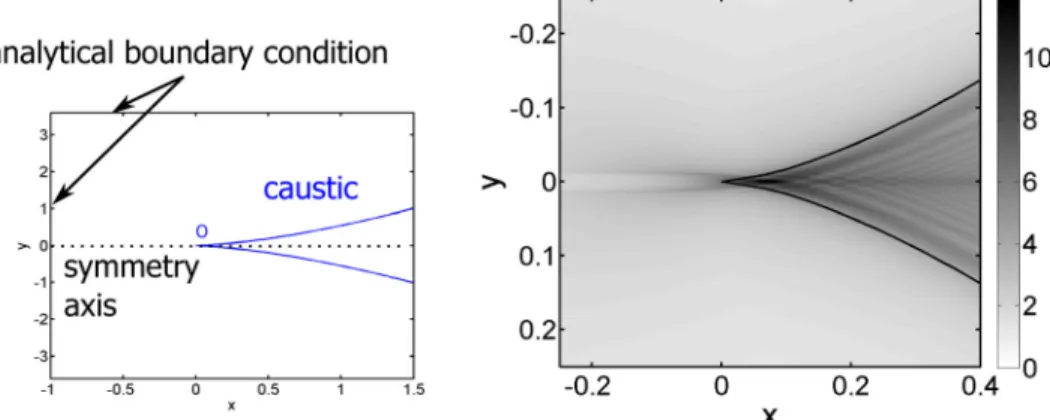
An analytical solution of this equation exists for the case of a caustic cusp [39] which is of particular interest here because: (1) it corresponds to a focused case such the ones we want to investi-gate; (2) the analytical solution is expressed in the time domain for a transient signal and not only in the frequency domain so it is well adapted to time domain solvers; and (3) for a shock wave, the analytical solution is singular (due to the ðs1Þ1=6 term) and therefore especially difficult to capture numerically. Indeed, for a focused shock, either nonlinearities or absorption is neces-sary for a finite solution.
An N-wave is used as an input waveform
FðsÞ ¼ s jsj 1 0 jsj>1
(
(25)
The following input time signal is imposed on the boundaries of the numerical domain surrounding the caustic cusp on a domain that is sufficiently large to support the caustic (as shown in Fig.2)
v xð ;y;sÞ ¼
F sþaðx;yÞyþa2 x;y
ð Þxa4 x;y ð Þ
ffiffiffiffiffiffiffiffiffiffiffiffiffiffiffiffiffiffiffiffiffiffiffiffiffiffiffiffi
j6a2ðx;yÞ xj
q (26)
Here, aðx;yÞ is the single real root of the polynomial 4a3 2axy¼0. This specific boundary condition is the exact boundary condition of a perfect cusp caustic of equation y2¼8x3=27 with a geometrical focus at the origin [39]. Note that in catastrophe theory [48], cusp caustics are second simplest after fold caustics. They are produced by an arbitrary curved wavefront that contains a local minimum in the radius of curvature. In this case, the geometrical parameteraintroduced in Eqs.(8)and(9)is
defined asa¼9R0ð0Þ2R000ð0Þ=8 withR0ðYÞ, which is the radius of curvature of the wavefront as a function of the transverse position Ywith a minimum atY¼0, andR000is its second-order derivative. In the frequency domain, solution of Eq.(24)with boundary con-dition Eq. (26) with FðsÞ ¼sinðsÞ is given by well-established Pearcey function [49].
The numerical solution was compared to this analytical solution on the nondimensional domain s2 ½3 4;x2 ½1 1, and y2 ½3:6 3:6withDx¼0:001 andDy¼0:001 (Nx¼2001 and
Ny¼7201). The sampling of the time domain is performed with
three valuesDs¼103;Ds¼5:103, andDs¼104, so, respec-tively,Ns¼7001;Ns¼14 001, andNs¼70 001. The right plot
in Fig.2shows the maximum particle velocity at each spatial grid point. Due to focusing effects, the incoming N-wave is amplified by over a factor of 10. The two characteristic branches of the caustic cusp are visible, as well as a complex interference pattern near the cusp. As expected, the position of the maximum of the amplitude is shifted slightly away from the geometrical focus (located at 0 on the y axis) because of diffraction effects. This shift varies with frequency as a function of x01=2 as given by Eq.(8). It is only at the high-frequency limit that the position of the focus corresponds to the geometrical focusx¼y¼0. These results qualitatively demonstrate that the numerical scheme suc-cessfully describes these challenging caustic cusps.
A quantitative validation is shown in Fig.3(a), which compares the computed waveform to the analytical solution [39] at the geometrical cusp. The numerical solution closely follows the ana-lytical result, including the overall signal shape and the two sharp peaks that occur as a result of focusing of the two shocks in the input N-wave. However, the analytical solution is singular at these two peaks since the shocks have an infinite frequency content. These singularities cannot be reproduced numerically, and the error is examined in more detail by zooming in on the first shock, which is shown in Fig.3(b). As expected, better agreement with the analytical singular solution is obtained by refining the time discretization. The numerical dissipation spreads out the shock slightly and it bounds the peak amplitudes to a finite value. The small oscillations following the focused shock are due to the second-order trapezoidal integration that introduces a small amount of numerical dispersion in the diffraction part of the algorithm.
Figure 3(c) compares the second- and first-order numerical solutions of Eq.(24). The first-order solution is computed with a rectangular discretization instead of a trapezoidal one. From this plot, it is clearly visible that the second-order scheme introduces much less numerical dissipation and better captures the sharp vari-ation around the shock. On the other hand, it induces a small amount of numerical dispersion that leads to oscillations behind the shock (barely visible in plot).
Fig. 2 Left: Schematic diagram of the domain of calculation used for the caustic cusp geome-try. O is the geometrical caustic point, at the origin. Right: maximum particle velocity determined by the numerical solution for a focused N-wave for the caseNs570,001. The
3.3 Two-Dimensional Nonlinear Validation: Guiraud’s Self-Similarity Law.There are no general solutions to Eq. (6) that can be used to validate the entire numerical scheme proposed in this paper. However, a strong confirmation of the numerical validity of the total algorithm can be obtained by examining self-similarity properties. Indeed, by ignoring the dissipation term in Eq.(6)(e.g., setting Abs¼0) and by carefully choosing the initial conditions, self-similar solutions can be found. The invariance of the numerical solution according to these scaling laws can then be used to establish the validity of the scheme. In acoustics, these self-similarity laws were established for quadratic nonlinearities, first for fold [50] and then for cusp caustics [39]. They are estab-lished here for cubic nonlinearities.
The input signal in the boundary condition (Eq.(27)) is chosen to be a step shock, which has an undefined characteristic time and is inherently invariant with scaling
FðsÞ ¼ 0 s0 1 s>0
(27)
Self-similarity is established by introducing the new scaled var-iables (denoted with an overbar)
v¼c1=4v x¼c1=2
x y¼c3=4y
s¼cs a¼c1=4a
8 > > > > > < > > > > > :
(28)
which subsequently make Eq.(15)and the boundary conditions in Eq.(26)independent of the amplitude parameterc. Physically, the first line in Eq.(28) shows that the focused velocity field has a power 1/2 dependence on the amplitude of the input field. Note that this is different from the compression wave case with quad-ratic nonlinearities, for which this power is 2/3 [39]. As expected, increasing the order of the nonlinearity leads to larger deviation from the linear case (which has a power of 1).
Self-similarity is verified numerically by solving Eq.(6)for an inviscid medium and its associated boundary conditions in Eq. (26) for different values of the parameterc. The numerical simulation is performed on a fixed domain defined by the dimen-sionless variablesðx;y;sÞfor the different values of the parameter
c. The number of points in the grid is allowed to increase withc
according to Eq. (28). The mesh parameters are summarized in Table1.
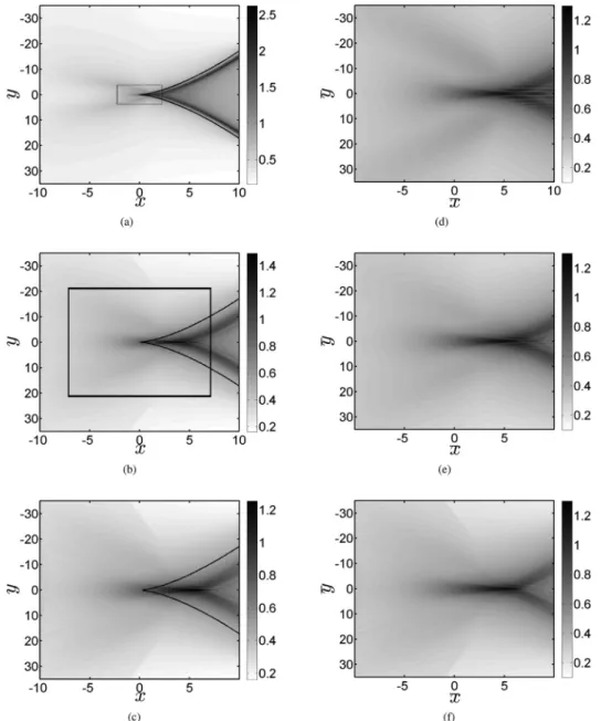
The solutions are then rescaled according to the self-similar variables in Eq.(28). This entire rescaling process is graphically illustrated in Fig.4for three values ofc. The images in the left column are the direct simulation calculated on the fixed domain. The images in the right column are rescaled by the self-similar variables. This allows a direct comparison of the simulations for different values of c. Note that c¼1 is used as the reference domain. This self-similar domain is outlined by a rectangle on the left column. Images in the right column should theoretically be identical. Consistent with this prediction, the images show that the numerical scheme satisfies the nonlinear self-similarity property. For instance, the shape of the focused field, the location of the maximum of velocity, and its amplitude are clearly similar for Fig. 3 Top left: comparison between the analytical solution (solid line) and numerical
different values of c. Nevertheless, the second-order numerical scheme introduces some numerical dispersion in the diffraction operator, as described in Sec.3.2. This leads to small oscillations behind the caustic, which break the perfect self-similarity of the
numerical results (these oscillations are difficult to observe in the images).
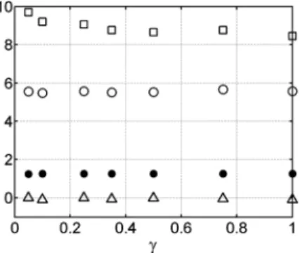
Figure5shows the position, time, and amplitude of the maxi-mum of the velocity field, rescaled according to their respective self-similar transformations (Eq.(28)), for a range of values ofc
between 0.05 and 1. Note that the location of the maximum is located on they¼0 axis due to symmetry, but not at the geometri-cal focusx¼0 due to diffraction and nonlinear effects.
In the ideal case, each variable would be independent ofcand would thus lay on a horizontal line. The positions and amplitude of the focal point shown in Fig.5closely follow the self-similarity law. There is, however, a slight deviation (around 10%) from this law for the time variable (squares) for low values ofc. Figure6 illustrates the mechanism behind this discrepancy. It shows the computed time waveforms rescaled in the self-similar variables, at the point of maximum amplitude forc2 ½0:05;1. Preceding the shock front, there is a nonphysical low slope region that clearly Table 1 Step size and number of points of each parameter
used for each parameterc
c (Dx,Nx) (Dy,Ny) (Dt,Nt)
0.05 (0.005, 3976) (0.0190, 3678) (0.0075, 8001)
0.1 (0.0071, 2811) (0.0320, 2187) (0.0150, 4001)
0.25 (0.0113, 1778) (0.0636, 1100) (0.0375, 1601)
0.35 (0.0133, 1503) (0.0819, 855) (0.0525, 1143)
0.5 (0.0159, 1258) (0.1070, 655) (0.0750, 801)
0.75 (0.0195, 1027) (0.1451, 483) (0.1125, 534)
1 (0.0225, 889) (0.1800, 389) (0.1500, 401)
deviates from the expected unperturbed valuev¼0. This precur-sor is due to numerical dispersion in the diffraction part of the algorithm and the numerical dissipation introduced by the nonlin-ear term—both tend to spread out the high-frequency content of the signal. This may explain the small error in the self-similarity of the time variable, which is more sensitive to dispersion errors. Another possible source of error is that the boundary conditions are imposed on a fixed domain while theoretically they are applied at an infinite distance. Therefore, the condition of large distance for the boundary conditions is better satisfied for numerical simu-lations with small values ofc. Nevertheless, the overall variability is comparatively low. The algorithm thus respects the predicted self-similarity scaling and is validated in the strongest possible in the absence of an analytical solution.
4
Nonlinear Focused Shear Waves in Brain
4.1 Model Configuration.The validated simulation tool was used to determine how focused shear shock waves can form in the brain. The initial conditions for this simulation were obtained from an X-ray computed tomography image of an anonymous human skull. The simulation was performed in two dimensions in a plane corresponding to a horizontal cut of the parietal bone (see Fig.7) at the level of the forehead. A globally concave portion of the parietal bone was selected for investigation. To avoid pixela-tion effects, the interior surface of the skull was interpolated with a fifth-order polynomial spline method that was then used to define the emitted wavefront. However, due to the retarded time formulation of Eq.(4), the simulation can only support initial con-ditions that are defined on a planar surface. Therefore, the source used in the simulation was calculated with a time-shifting method that projects the interior skull surface onto the source plane shown in Fig.7. Each point of the source plane emits a wave with a phase
shifted by DTðYÞ ¼DXðYÞ=cT, where DXðYÞ is the distance between the point ofYaxis and the source plane shown in Fig.7. The geometry investigated here approaches a half-angle of 50 deg and is therefore beyond the limit of validity of the parabolic approximation, which is 18 deg. However, the point of this study is to demonstrate that nonlinear effects can be dominant in regimes that are consistent with traumatic brain injury. For the purposes of this study, we are therefore willing to accept a para-bolic approximation, which, in terms of diffraction, changes slightly the location of the focus, to increase the accuracy of shock wave modeling.
The linear elastic material properties of the brain have been investigated by many authors, a recent synthesis being provided by Chatelin et al. [51]. These studies indicate a large variability depending on the measurement process (for instance, in vitro or in vivo) and whether human or animal (porcine, bovine, calf, monkey, etc.). Age dependence remains poorly understood. Shear behavior of brain matter is clearly viscoelastic with relaxation processes [52,53]. White matter has been shown anisotropic, while gray matter turns out isotropic [54,55]. For instance, in their FE linear modeling of brain response, Zhang et al. [28] used val-ues found in Ref. [56] with the shear modulus varying between 6:4 kPa (long time) and 34 kPa (short time) for the gray matter and between 7:8 kPa and 41 kPa for the white matter.
The nonlinear parametersðA;D;andbÞhave been measured in gelatin phantoms, with acoustoelastic methods to obtain the third-order elastic constantA[12] and by determination of the level of third harmonic to obtain the nonlinear parameterb[13]. In these last two references, the medium was an agar/gelatin gel with 5% gelatin concentration and 3% agar. Its shear modulus is in the range of 6:3560:04 kPa and 6:660:6 kPa, which is very similar to the long time shear modulus measured by Shuck and Advani [56] in the brain. The gel density is equal to 1.04, the same value reported by Zhang et al. [28] for both white and gray matter. This leads to a shear wave speed cT¼2:5260:12 m=s. The gelatin phantom nonlinear parameter was measured to be b¼460:5 [13]. The absorption coefficient at a frequency off0¼100 Hz was measured asaðf0Þ ¼17 Np=m. The absorption law as a function of frequency was empirically determined to be simply propor-tional to frequency [3]
að Þ ¼f að Þf0 f
f0 (29)
Consequently, Gol’dberg number, which is a ratio of the nonli-nearity and attenuation, is independent of frequency and depends only on the amplitude.
Very recently, the nonlinear parameters have also been measured in fresh porcine brain using acoustoelastographic meas-urements of linear shear wave propagation in combination with solutions of an inverse problem [57]. The reported values are Fig. 5 Values of self-similar variablesx (circle),y(triangle),v
(disk), and2t (square) of the point of maximum amplitude for different values ofc. In the ideal case, each value would follow a horizontal line.
l¼2:460:5 kPa;A¼ 13:567:9 kPa, and D¼5:961:6 kPa. Unfortunately, the variability in these measurements is large in terms of b which according to these results can vary between 3.55 and 5.21. Note that negative values of b correspond to shear softening and positive values to shear stiffening nonlinear-ity. Only the latter phenomenon has been observed directly in gel-atin [3]. There is currently no direct experimental observation of shear shock waves in brain. We therefore choose to use the meas-urements reported for gelatin because (a) they fall within the range reported for brain and (b) they respect the observed shock wave physics in soft solids. The values used in subsequent simula-tions are thusl¼6:6 kPa andb¼4.
4.2 Blunt Impact.In this section, a blunt head impact that is focused in by the skull into the brain was simulated. A common criterion in the literature to quantify head impact is the so-called head injury criterion (HIC) [58] proposed by the U.S. National Highway Traffic Safety Administration
HIC¼ðt2t1Þ 1 t2t1
ðt2
t1 adt
" #2:5
(30)
wheret1is the initial time of contact,t2is the end time of contact, andais the head acceleration. Typical values for the impact dura-tion t2t1 are less than 15 ms and HIC values go up to a few thousands [30,59]. Such values correspond to trauma resulting either from well-documented motorcyclist accidents [60] or from football head injuries, in both cases with helmets, that lead to severe diffuse axonal injuries. This corresponds to frequencies larger than 66 Hz, velocities of the order of a few meters per sec-ond and accelerations on the order of 10g. Higher accelerations of several hundreds of g are reported in cases of ballistic impact
[61]. Hence, for typical simulations, we chose as input waveform a sinusoidal signal with a center frequency of f0¼100 Hz, a single cycle envelope (see Fig.8(a)), and an initial amplitude,V0, chosen to be lower than 2 m=s. Note, however, that such values have been observed for external head motion. The transfer func-tion to the brain tissue shearing is a complex process [28] that depends on the blunt impact orientation and location, the skull mechanical properties, and the skull–brain interface that itself is composed of three layers (dura, arachnoid, and pia maters). Modeling such process is not in the scope of the present study and for simplicity, we assumed a perfect transfer but with unknown velocity amplitude. Hence, a parametric study was performed by varying this velocity.
To ensure the convergence of the simulation, we used 400 points per wavelengths in time. The mesh on the x axis was chosen according to the stability condition (Eq.(22)), so that the simulations requiredNx¼3155 points on the xaxis with a step
size Dx¼2:3777105m. The y axis was discretized with Ny¼690 points and a step sizeDy¼2:6276104m. Only the
central 490y-points are shown in the following results. The lateral extent of the numerical domain is about 18 cm, which is larger than the size of the selected part of the brain (about 12 cm). Com-bined with the geometrical focusing effect, this prevented lateral reflections from interfering with the focal zone.
Figure9shows the total energy, acceleration [61,62], and shear stress [63] for initial condition amplitudes of 0:05 m=s;0:6 m=s, and 1 m=s. Figures9(a)–9(c)show the total energyEof the signal calculated asE¼q=2PkðVjn;kÞ
2
Dtat each point of the numerical domain. The time plot at the focus is shown for each of these three amplitudes in Fig.8(b). Figures9(d)–9(f)show maps of the maxi-mum acceleration at each point of the spatial domain for the three initial velocities. Since absorption is empirical (see Eq.(29)), only the elastic part of the shear stress was calculated. It is defined as Fig. 7 CT of a human head. Dark gray: bone. Light gray: soft tissues. Left: vertical central cut. The horizontal line indicates the horizontal cut. Middle: horizontal cut. The arrow indicates the selected parietal area. Right: the selected parietal area. The doted line indicates the input plane for numerical simulations.
r31¼l
@u3
@x1þ lþ A 2þD
@u3
@x1
3
(31)
The numerical value forr31is calculated according to Eq.(31), by changing the variables from ðt;x1Þ to ðs;XÞ. The numerical output of the velocity field is differentiated by a first-order scheme so that
rn jk¼
l
cT Vjn;kþl
Xk
K¼0
Vnj;KVn
1 j;K
Ds
DX
2b
3c3 T
Vjn;k
3
(32)
Note that in agreement with Eq.(4), only the leading nonlinear term involving partial derivative with respect to retarded time is retained. The shear stress is shown in Figs.9(g)–9(i).
All the images in Fig.9show a clear focal spot that is observ-able at a depth of about x¼0:04 m. For an initial velocity V0ⱗ0:5 m=s, there is no shock at the focal point. Shock waves appear for higher velocities, first in the negative phase of the shear wave (see the caseV0¼0:6 m=s), then in the positive phase. This shock wave formation distance can be calculated analytically for a plane sinusoidal wave. For the three considered velocities, this distance is, respectively, 2:54 m;0:018 m, and 0:0064 m. Attenua-tion and diffracAttenua-tion slightly lengthen the plane wave estimates. Nevertheless, the orders of magnitude are correct. Therefore,
compared to the 0:04 m geometrical focus, the three initial condi-tions correspond to a shock formation distance well past the focus, near the focus, and well before the focus. This leads to three dis-tinct types of behavior.
In the first case, shown as the left column in Fig.9, no shock waves form and the propagation behavior is quasi-linear. There is therefore some focal gain which is reduced by attenuation. Over-all, there are no strong variations in the fields. In the second case, in the middle column of Fig.9, where the shock formation dis-tance and focal disdis-tance are approximately the same, there is a dramatic difference between the behavior at the focus and the rest of the field. In particular, Fig.9(e)shows that the maximum accel-eration in the focal zone is much higher than anywhere else. The acceleration at the initial condition surface is 60 m=s2, and it is over 800 m=s2 in the focal region. This is due to the focal gain and shock formation which act together in a small region and can thus easily overcome attenuation to generate very high local accelerations. In the third case, the right column of Fig.9, the shock forms in the first few millimeters of propagation, which cor-responds to a small fraction of the wavelength. There is therefore a shear shock wave propagating in whole region between the ini-tial condition surface, on the left, and beyond the focal zone. This behavior is particularly clear from the acceleration plot, see Fig.9(f).
Generally, the results indicate a very efficient increase in maxi-mum acceleration as soon as shock waves appear. Indeed, shock Fig. 9 Maximum of energy (top), acceleration (middle), and shear stressr31(bottom) on the calculation domain for initial
waves in inviscid media would lead to an infinite acceleration. Here, acceleration remains finite due to the smoothing effects of absorption. Nevertheless, very high local acceleration values can be reached, up to a few thousand ofg’s, at the shock front. These high accelerations can be localized in a small region due to focusing.
Focusing in terms of acceleration is much more efficient than in terms of energy or shear stress. The latter two behave in a similar fashion in the sense that there is a clear focusing effect but the local variations in the focal zone are not much larger than in the near field.
The transition from the quasi-linear regime to the shock regime can be characterized more finely by considering additional values in the initial condition velocity. Figure10shows the maximum amplitudes of velocity, acceleration, and shear stress at the focal point, for initial velocities between 0:05 m=s and 1 m=s. The left plot of Fig. 10 shows that when the initial condition velocity increases, the maximum velocity at the focus increases in a linear fashion up to approximately 0:5 m=s. Beyond these values, shocks are observed at the focus and the velocity increases in a sublinear fashion. This is due to energy loss at the shock front. For accelera-tion, shown in the middle plot of Fig.10, the linear regime ends at approximately 0:3 m=s. This is due to the fact that a shock is not required to increase the acceleration, rather nonlinear steepening increases the acceleration. For initial velocities of 0:5 m=s, when shocks form, there is a dramatic increase in the maximum acceler-ation observed at the focus. Beyond values of approximately 0:9 m=s, there is a saturation effect which corresponds to nonlin-ear dissipation. The behavior of the shnonlin-ear stress, shown on the right, is similar but with much less amplification compared to the acceleration.
5
Conclusion
For soft tissues, the shear wave velocity is so low (on the order of a few meters per second) that nonlinear effects are very intense and shocks form over distances that are less than a wavelength (on the order of a few centimeters). We have developed models and simulation tools that can describe this relatively unexplored behavior to investigate how the spherical skull geometry can influ-ence shear shock formation in the brain.
The results were presented as function of velocities that are rel-evant to TBI, i.e., brain velocities between 0:05 m=s and 2 m=s. Within this parameter, range three distinct regimes were observed. First, at low amplitudes the shear wave propagation is practically linear. There are therefore some focusing effects due to the skull geometry, but no large differences between the focal region and the rest of the field for acceleration, energy, or shear stress. Sec-ond, the regime where the focal zone and shock wave formation distance are comparable exhibited dramatic differences between the focal zone and the rest of the field. In particular, for the 0:6 m=s case, the acceleration at the source was 60 m=s2 and at the focus it was 860 m=s2. This corresponds to an almost 15-fold
increase in the acceleration in a strongly localized area of the brain. This suggests that focused shear shock waves could be a mechanism that causes diffuse axonal injuries. Third, for large velocities, the shock formation distance is a fraction of a wave-length (a few millimeters). Therefore, shocks form near the source and continue to propagate past the focus. Energy at these high dis-plays a saturation effect because of the additional dissipation through shocks. For the largest input velocity values, nonlinear-ities are so strong that the wave is nonlinearly starting from the skull surface.
This study demonstrates the importance of nonlinear effects and the shock wave formation and focusing in the brain volume. Because brain material parameters remain uncertain, the constitu-tive parameters of gelatin were used; behavior of shear waves in brain tissue might be qualitatively different. Since the simulations were performed in 2D, the focal effect may be underestimated compared to the 3D spherical skull geometry which has an even larger focal gain. Nevertheless, the study demonstrates a new potential mechanism for diffuse axonal injuries and tissue dam-age. Further studies will consider removing the paraxial approxi-mation, investigating other polarizations, and comparing the simulations with laboratory experiments.
Acknowledgment
The authors would like to acknowledge support from the NIH R01 NS091195-01.
References
[1] Catheline, S., Gennisson, J.-L., Tanter, M., and Fink, M., 2003, “Observation of Shock Transverse Waves in Elastic Media,” Phys. Rev. Lett., 91(16), p. 164301.
[2] Whitham, G., 1979,Lectures on Wave Propagation, Springer-Verlag, Berlin. [3] Catheline, S., Gennisson, J.-L., Delon, G., Fink, M., Sinkus, R., Abouelkaram,
S., and Culioli, J., 2004, “Measurement of Viscoelastic Properties of Homoge-neous Soft Solid Using Transient Elastography: An Inverse Problem Approach,”J. Acoust. Soc. Am.,116(6), pp. 3734–3741.
[4] Duck, F. A., 2013,Physical Properties of Tissues: A Comprehensive Reference Book, Academic Press, London.
[5] Sandrin, L., Tanter, M., Catheline, S., and Fink, M., 2002, “Shear Modulus Imaging With 2-D Transient Elastography,”IEEE Trans. Ultrason., Ferroe-lectr., Freq. Control,49(4), pp. 426–435.
[6] Hamilton, M., Ilinskii, Y., and Zabolotskaya, E., 2004, “Separation of Compres-sibility and Shear Deformation in the Elastic Energy Density (L),”J. Acoust. Soc. Am.,116(1), pp. 41–44.
[7] Destrade, M., and Ogden, R. W., 2010, “On the Third-and Fourth-Order Constants of Incompressible Isotropic Elasticity,”J. Acoust. Soc. Am.,128(6), pp. 3334–3343.
[8] Zabolotskaya, E., Hamilton, M., Ilinskii, Y., and Meegan, G. D., 2004, “Modeling of Nonlinear Shear Waves in Soft Solids,”J. Acoust. Soc. Am., 116(5), pp. 2807–2813.
[9] Wochner, M., Hamilton, M., Ilinskii, Y., and Zabolotskaya, E., 2008, “Cubic Nonlinearity in Shear Wave Beams With Different Polarizations,”J. Acoust. Soc. Am.,123(5), pp. 2488–2495.
[10] Kuznetsov, V., 1971, “Equations of Nonlinear Acoustics,” Sov. Phys. Acoust., 16(4), pp. 467–470.
[11] Jacob, X., Catheline, S., Genisson, J.-L., Barrie`re, C., Royer, D., and Fink, M., 2007, “Nonlinear Shear Wave Interaction in Soft Solids,”J. Acoust. Soc. Am., 122(4), pp. 1917–1926.
[12] Gennisson, J.-L., Renier, M., Catheline, S., Barrie`re, C., Bercoff, J., Tanter, M., and Fink, M., 2007, “Acoustoelasticity in Soft Solids: Assessment of the Non-linear Shear Modulus With the Acoustic Radiation Force,”J. Acoust. Soc. Am., 122(6), pp. 3211–3219.
[13] Renier, M., Gennisson, J.-L., Barrie`re, C., Royer, D., and Fink, M., 2008, “Fourth-Order Shear Elastic Constant Assessment in Quasi-Incompressible Soft Solids,”Appl. Phys. Lett.,93(10), p. 101912.
[14] Pinton, G., Coulouvrat, F., Gennisson, J.-L., and Tanter, M., 2010, “Nonlinear Reflection of Shock Shear Waves in Soft Elastic Media,”J. Acoust. Soc. Am., 127(2), pp. 683–691.
[15] Hamhaber, U., Klatt, D., Papazoglou, S., Hollmann, M., Stadler, J., Sack, I., Bernarding, J., and Braun, J., 2010, “In Vivo Magnetic Resonance Elastography of Human Brain at 7 T and 1.5 T,” J. Magn. Reson. Imaging, 32(3), pp. 577–583.
[16] Johnson, C. L., McGarry, M. D., Houten, E. E., Weaver, J. B., Paulsen, K. D., Sutton, B. P., and Georgiadis, J. G., 2013, “Magnetic Resonance Elastography of the Brain Using Multishot Spiral Readouts With Self-Navigated Motion Correction,”Magn. Reson. Med.,70(2), pp. 404–412.
[17] Fu, M., Barlaz, M. S., Shosted, R. K., Liang, Z.-P., and Sutton, B. P., 2015, “High-Resolution Dynamic Speech Imaging With Deformation Estimation,” 37th Annual International Conference of the IEEE on Engineering in Medicine and Biology Society (EMBC), Milan, Italy, Aug. 25–29, pp. 1568–1571. [18] Walker, W. F., and Trahey, G. E., 1995, “A Fundamental Limit on Delay
Estimation Using Partially Correlated Speckle Signals,”IEEE Trans. Ultrason., Ferroelectr., Freq. Control,42(2), pp. 301–308.
[19] Pinton, G. F., Dahl, J. J., and Trahey, G. E., 2006, “Rapid Tracking of Small Displacements With Ultrasound,”IEEE Trans. Ultrason., Ferroelectr., Freq. Control,53(6), pp. 1103–1117.
[20] Pinton, G., Gennisson, J.-L., Tanter, M., and Coulouvrat, F., 2014, “Adaptive Motion Estimation of Shear Shock Waves in Soft Solids and Tissue With Ultra-sound,” IEEE Trans. Ultrason., Ferroelectr., Freq. Control, 61(9), pp. 1489–1503.
[21] Hart, T., and Hamilton, M., 1988, “Nonlinear Effects in Focused Sound Beams,”J. Acoust. Soc. Am.,84(4), pp. 1488–1496.
[22] Averkiou, M., and Hamilton, M., 1997, “Nonlinear Distortion of Short Pulses Radiated by Plane and Focused Circular Pistons,”J. Acoust. Soc. Am.,102(5), pp. 2539–2548.
[23] Marchiano, R., Coulouvrat, F., and Grenon, R., 2003, “Numerical Simulation of Shock Wave Focusing at Fold Caustics, With Application to Sonic Boom,” J. Acoust. Soc. Am.,114(4), pp. 1758–1771.
[24] Marchiano, R., Thomas, J.-L., and Coulouvrat, F., 2003, “Experimental Simula-tion of Supersonic Superboom in a Water Tank: Nonlinear Focusing of Weak Shock Waves at a Fold Caustic,”Phys. Rev. Lett.,91(18), p. 1843901. [25] Chen, Y., and Ostoja-Starzewski, M., 2010, “MRI-Based Finite Element
Mod-eling of Head Trauma: Spherically Focusing Shear Waves,” Acta Mech., 213(1–2), pp. 155–167.
[26] Shugar, T., 1977, “A Finite Element Head Injury Model,” Department of Trans-portation, National Highway Traffic Safety Administration, Report No. DOT HS-289-3-550.
[27] Hosey, R., and Liu, Y., 1982, “A Homeomorphic Finite Element Model of the Human Head and Neck,”Finite Elements in Biomechanics, Wiley, New York, pp. 379–401.
[28] Zhang, L., Yang, K., and King, A., 2001, “Comparison of Brain Responses Between Frontal and Lateral Impacts by Finite Element Modeling,”J. Neuro-trauma,18(1), pp. 21–30.
[29] Taylor, P. A., and Ford, C., 2009, “Simulation of Blast-Induced Early-Time Intracranial Wave Physics Leading to Traumatic Brain Injury,”ASME J. Bio-mech. Eng.,131(6), p. 61007.
[30] Chatelin, S., Deck, C., Renard, F., Kremer, S., Heinrich, C., Armspach, J.-P., and Willinger, R., 2011, “Computation of Axonal Elongation in Head Trauma Finite Element Simulation,” J. Mech. Behav. Biomed. Mater., 4(8), pp. 1905–1919.
[31] Nyein, M., Jerusalem, A., Radovitzky, R., Moore, D., and Noels, L., 2008, “Modeling Blast-Related Brain Injury,” MIT, Cambridge, MA,DTIC Docu-ment No. ADA504193.
[32] Moore, D., Jerusalem, A., Nyein, M., Noels, L., Jaffee, M., and Radovitzky, R., 2009, “Computational Biology—Modeling of Primary Blast Effects on the Cen-tral Nervous System,”Neuroimage,47, pp. T10–T20.
[33] Mendis, K., 1992, “Finite Element Modeling of the Brain to Establish Diffuse Axonal Injury Criteria,”Ph.D. thesis, The Ohio State University, Columbus, OH. [34] Brands, D., Peters, G., and Bovendeerd, P., 2004, “Design and Numerical
Implementation of a 3-D Non Linear Viscoelastic Constitutive Model for Brain Tissue During Impact,”J. Biomech.,37(1), pp. 127–134.
[35] Landau, L., and Lifshitz, E., 1959, “Course of Theoretical Physics,”Theory and Elasticity, Vol. 7, Pergamon Press, Oxford, UK.
[36] Khokhlova, V., Ponomarev, A., Averkiou, M., and Crum, L., 2006, “Nonlinear Pulsed Ultrasound Beams Radiated by Rectangular Focused Diagnostic Trans-ducers,”Acoust. Phys.,52(4), pp. 481–489.
[37] Yang, L., Chen, Y.-Y., and Yu, S.-T. J., 2013, “Viscoelasticity Determined by Measured Wave Absorption Coefficient for Modeling Waves in Soft Tissues,” Wave Motion,50(2), pp. 334–346.
[38] Lee, Y.-S., and Hamilton, M., 1995, “Time-Domain Modeling of Pulsed Finite-Amplitude Sound Beams,”J. Acoust. Soc. Am.,97(2), pp. 906–917. [39] Coulouvrat, F., 2000, “Focusing of Weak Acoustic Shock Waves at a Caustic
Cusp,”Wave Motion,32(3), pp. 233–245.
[40] Strang, G., 1968, “On the Construction and Comparison of Difference Schemes,”SIAM J. Numer. Anal.,5(3), pp. 506–517.
[41] Loubeau, A., and Coulouvrat, F., 2009, “Effects of Meteorological Variability on Sonic Boom Propagation From Hypersonic Aircraft,”AIAA J.,47(11), pp. 2632–2641.
[42] Dagrau, F., Renier, M., Marchiano, R., and Coulouvrat, F., 2011, “Acoustic Shock Wave Propagation in a Heterogeneous Medium: A Numerical Simulation Beyond the Parabolic Equation,”J. Acoust. Soc. Am.,130(1), pp. 20–32. [43] Yang, X., and Cleveland, R., 2005, “Time Domain Simulation of Nonlinear
Acoustic Beams Generated by Rectangular Pistons With Application to Har-monic Imaging,”J. Acoust. Soc. Am.,117(1), pp. 113–123.
[44] Coulouvrat, F., 2009, “A Quasi-Analytical Shock Solution for General Nonlin-ear Progressive Waves,”Wave Motion,46(2), pp. 97–107.
[45] McDonald, B., and Ambrosiano, J., 1984, “High-Order Upwind Flux Correction Methods for Hyperbolic Conservation Laws,” J. Comput. Phys., 56(3), pp. 448–460.
[46] Boris, J., and Book, D., 1973, “Flux-Corrected Transport. I. SHASTA, A Fluid Transport Algorithm That Works,”J. Comput. Phys.,11(1), pp. 38–69. [47] LeVeque, R. J., 2002, Finite Volume Methods for Hyperbolic Problems,
Cambridge University Press, Cambridge.
[48] Marston, P., 1992, “Geometrical and Catastrophe Optics Methods in Scattering,”Physical Acoustics, Vol. XXI, Academic Press, San Diego, CA, pp. 1–234.
[49] Pearcey, T., 1946, “The Structure of an Electromagnetic Field in the Neigh-bourhood of a Cusp of a Caustic,”Philos. Mag.,37(268), pp. 311–317. [50] Guiraud, J.-P., 1965, “Acoustique Geometrique, Bruit Balistique des Avions
Supersoniques et Focalisation,” J. Mecanique,4, pp. 215–267.
[51] Chatelin, S., Constantinesco, A., and Willinger, R., 2010, “Fifty Years of Brain Tissue Mechanical Testing: From In Vitro to In Vivo Investigations,” Biorheo-logy,47(5), pp. 255–276.
[52] Arbogast, K., Meaney, D., and Thibault, L., 1997, “Biomechanical Characteri-zation of the Constitutive Relationship for the Brainstem,” SAE Technical Paper No. 952716.
[53] Bilston, L., Liu, Z., and Phan-Thien, N., 1997, “Linear Viscoelastic Properties of Bovine Brain Tissue in Shear,”Biorheology,34(6), pp. 377–395.
[54] Ning, X., Zhu, Q., Lanir, Y., and Margulies, S., 2006, “A Transversely Isotropic Viscoelastic Constitutive Equation for Brainstem Undergoing Finite Deformation,”ASME J. Biomech. Eng.,128(6), pp. 925–933.
[55] Prange, M., Meaney, D., and Margulies, S., 2000, “Defining Brain Mechanical Properties: Effects of Region, Direction, and Species,”Stapp Car Crash J.,44, pp. 205–213.
[56] Shuck, L., and Advani, S., 1972, “Rheological Response of Human Brain Tis-sue in Shear,”ASME J. Basic Eng.,94(4), pp. 905–911.
[57] Jiang, Y., Li, G., Qian, L.-X., Liang, S., Destrade, M., and Cao, Y., 2015, “Measuring the Linear and Nonlinear Elastic Properties of Brain Tissue With Shear Waves and Inverse Analysis,”Biomech. Model. Mechanobiol.,14(5), pp. 1–10.
[58] Gadd, C., 1966, “Use of a Weighted-Impulse Criterion for Estimating Injury Hazard,” SAE Technical Paper No. 660793.
[59] Greenwald, R., Gwin, J., Chu, J., and Crisco, J., 2008, “Head Impact Severity Measures for Evaluating Mild Traumatic Brain Injury Risk Exposure,” Neuro-surgery,62(4), pp. 789–798.
[60] Chinn, B., Doyle, D., Otte, D., and Schuller, E., 1999, “Motorcyclists Head Injuries: Mechanisms Identified From Accident Reconstruction and Helmet Damage Replication,” International Research Council on the Biomechanics of Injury Conference (IRCOBI), Vol. 27, pp. 53–71.
[61] Raymond, D., Van Ee, C., Crawford, G., and Bir, C., 2009, “Tolerance of the Skull to Blunt Ballistic Temporo-Parietal Impact,” J. Biomech., 42(15), pp. 2479–2485.
[62] Shridharani, J. K., Wood, G. W., Panzer, M. B., Capehart, B., Nyein, M. K., Radovitzky, R. A., and Bass, C. R., 2012, “Porcine Head Response to Blast,” Front. Neurol.,3, p. 70.
![Figure 9 shows the total energy, acceleration [61,62], and shear stress [63] for initial condition amplitudes of 0:05 m=s; 0:6 m=s, and 1 m=s](https://thumb-us.123doks.com/thumbv2/123dok_us/8297694.2197477/9.918.109.819.65.236/figure-shows-energy-acceleration-stress-initial-condition-amplitudes.webp)

