27be745d9d3b62ce94c579433882c3f509d225fb.pdf

LETTER • OPEN ACCESS

Carbon reductions and health co-benefits from US

residential energy efficiency measures

To cite this article: Jonathan I Levy et al 2016 Environ. Res. Lett. 11 034017

View the article online for updates and enhancements.

Related content

Air quality and climate benefits of long-distance electricity transmission in China Wei Peng, Jiahai Yuan, Yu Zhao et al.

-Health and climate benefits of offshore wind facilities in the Mid-Atlantic United States

Jonathan J Buonocore, Patrick Luckow, Jeremy Fisher et al.

-Impact of warmer weather on electricity sector emissions due to building energy use

Paul Meier, Tracey Holloway, Jonathan Patz et al.

-Recent citations

Impacts of air pollutants from rural Chinese households under the rapid residential energy transition Guofeng Shen et al

-A strong relative preference for wind turbines in the United States among those who live near them

Jeremy Firestone and Hannah Kirk

-The air quality-related health benefits of energy efficiency in the United States David Abel et al

Environ. Res. Lett.11(2016)034017 doi:10.1088/1748-9326/11/3/034017

LETTER

Carbon reductions and health co-bene

fi

ts from US residential energy

ef

fi

ciency measures

Jonathan I Levy1

, May K Woo1

, Stefani L Penn1

, Mohammad Omary2

, Yann Tambouret3

, Chloe S Kim1

and

Saravanan Arunachalam2

1 _{Boston University School of Public Health, 715 Albany St. T4W, Boston, MA 02118, USA}

2 _{Institute for the Environment, University of North Carolina at Chapel Hill, 100 Europa Drive Suite 490, Chapel Hill, NC 27517, USA} 3 _{Research Computing Services, Boston University, 111 Cummington Mall, Boston, MA 02215, USA}

E-mail:[email protected]

Keywords:air pollution, energy efficiency, carbon dioxide, power plant, residential, public health

Supplementary material for this article is availableonline

Abstract

The United States

(

US

)

Clean Power Plan established state-speci

fi

c carbon dioxide

(

CO

emissions

reduction goals for fossil fuel-

fi

red electricity generating units

(

EGUs

)

. States may achieve these goals

through multiple mechanisms, including measures that can achieve equivalent CO

reductions such

as residential energy ef

fi

ciency, which will have important co-bene

fi

ts. Here, we develop

state-resolution simulations of the economic, health, and climate bene

fi

ts of increased residential

insulation, considering EGUs and residential combustion. Increasing insulation to International

Energy Conservation Code 2012 levels for all single-family homes in the US in 2013 would lead to

annual reductions of 80 million tons of CO

from EGUs, with annual co-bene

fi

ts including 30 million

tons of CO

from residential combustion and 320 premature deaths associated with criteria pollutant

emissions from both EGUs and residential combustion sources. Monetized climate and health

co-bene

fi

ts average $49 per ton of CO

reduced from EGUs

(

range across states: $12

–

$390

)

. State-speci

fi

c

co-bene

fi

t estimates can inform development of optimal Clean Power Plan implementation strategies.

Introduction

In August 2015, the United States Environmental Protection Agency(US EPA)issued the Final Rule for the Clean Power Plan [1], which established state-specific carbon dioxide (CO2) emissions reduction goals for fossil fuel-fired electricity generating units (EGUs). States may achieve these goals through multi-ple mechanisms, including source-specific emissions standards or measures that can achieve equivalent CO2reductions, such as residential energy efficiency.

Residential energy efficiency is an appealing approach for emissions reductions, given evidence of greater cost-effectiveness relative to other strategies

[2]. While studies have identified some of the eco-nomic benefits of energy efficiency as a CO2emissions reduction strategy, important co-benefits are often not considered in policy development. Such co-benefits include the influence of other air pollutants from EGUs on public health. Studies have shown that the air

pollution-related public health benefits of EGU con-trol strategies can be appreciable, with thousands of lives saved per year and an array of morbidity benefits for CO2 control strategies that include energy effi -ciency[3]. The monetary value of air pollution health benefits from EGU emissions reductions has been shown to be comparable in magnitude to the social cost of carbon(SCC)[4,5]. In addition, energy effi -ciency measures that influence heating and cooling (e.g., increased residential insulation or air sealing) would not only reduce emissions from EGUs, but would also reduce emissions of CO2and other air pol-lutants from direct residential combustion.

Although these pathways are well-recognized, models to date have not provided insight at the state level on the multifactorial benefits of specific residen-tial energy efficiency measures. Models of energy sav-ings associated with energy efficiency are readily available[6]but without extension to emissions and health co-benefits. Recent models examining the

OPEN ACCESS

RECEIVED

23 December 2015

REVISED

23 February 2016

ACCEPTED FOR PUBLICATION

23 February 2016

PUBLISHED

7 March 2016

Original content from this work may be used under the terms of theCreative Commons Attribution 3.0 licence.

Any further distribution of this work must maintain attribution to the author(s)and the title of the work, journal citation and DOI.

commercial sector incorporated social benefits at the state level related to both CO2emissions and other air pollutants[7], but focused only on electricity and nat-ural gas, calculated health benefits using estimates that relied on an atmospheric dispersion model with lim-ited secondary chemistry, and characterized average rather than marginal emission rates from the power grid. An older study of the residential sector estimated social benefits of increased residential insulation by extrapolating findings from a more complex atmo-spheric dispersion model and estimating marginal emission rates, but did not model all source locations directly or account for more complex patterns of elec-tricity dispatch[8]. Studies have applied more com-plex atmospheric models to evaluate air pollution benefits of energy efficiency or other interventions, but generally only at a national scale [3]. To our knowledge, no studies have incorporated all of the ele-ments needed to accurately estimate social benefits of residential energy efficiency measures or to quantify co-benefits of residential energy efficiency measures targeting CO2at the state level.

In this study, we develop and apply a comprehen-sive and integrated model of the economic, climate, and public health benefits of increased insulation as an example of a state-level residential energy efficiency measure. We construct detailed simulations of the state-level energy savings associated with increasing residential insulation for all single-family homes in the continental US in 2013 to levels consistent with the 2012 International Energy Conservation Code (IECC). We estimate emissions reductions by state from both EGUs and residential combustion, and we link these emissions reductions with atmospheric chemistry-transport modeling approaches which allow us to isolate the contribution from individual emitted pollutants, source types, and states to ambient air pollution. We estimate the resulting public health benefits of reductions in ozone andfine particulate matter(PM2.5)concentrations and we monetize both health benefits and CO2emission reductions. We pre-sent our central estimates and characterize uncertainty across multiple model components. These outputs allow us to quantify the co-benefits of state-level energy efficiency strategies targeting CO2 emissions from EGUs, and to compare the health and climate benefits with the economic benefits associated with residential energy efficiency.

Methods

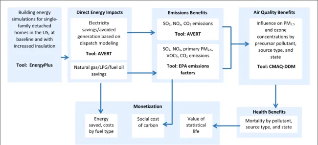
Our simulation model consists offive primary compo-nents (figure 1). We describe each of these model components in the sections that follow, with more detail about our energy simulation modeling and atmospheric modeling in supplementary data.

Energy simulation modeling

We simulated building-wide energy consumption using high-performance computing techniques with an energy simulation program(EnergyPlus)which has been extensively applied and validated in the peer-reviewed literature[9–12]. We began with EnergyPlus building prototypes developed by Pacific Northwest National Laboratory (PNNL) and made available through the Building Energy Codes Program of the US Department of Energy[13]. We then modified these prototypes to correspond with single-family detached homes representative of the US housing stock, using microdata from the 2009 Residential Energy Con-sumption Survey(RECS; see supplementary data).

We ran EnergyPlus for each home with current insulation and with increased insulation in the wall, ceiling, and floor consistent with the state-specific 2012 IECC. To calculate the benefits of increased resi-dential insulation by state, we selected the RECS tem-plates assigned to each state and calculated the differences in hourly energy consumption between the existing home and post-retrofit home. We then esti-mated the state-level benefits by using the RECS sam-ple weight for each home but rescaling to represent the total number of single-family homes in each state, as derived from 2009 to 2013 American Community Survey estimates.

Because of the need to edit and simulate energy consumption for tens of thousands of templates, we developed code in Python to batch edit, process, and run homes in EnergyPlus. We utilized Eppy [14], a previously developed Python library for processing EnergyPlus inputs and outputs, for the batchfile edits. We ran the simulations on the Shared Computing Cluster, a heterogeneous Linux cluster at Boston University.

We conducted two primary sensitivity analyses. First, given the possibility of systematic bias in Energy-Plus, we developed calibration factors by reportable domain(state or state aggregates), fuel type(electricity, natural gas, fuel oil, LPG/propane), and usage cate-gory(heating, cooling, all other)by comparing simu-lated baseline energy consumption with corresponding values from RECS. We used the cali-brated values for our primary estimates but tested the sensitivity of ourfindings to the use of uncalibrated values. Second, because air tightness can greatly infl u-ence heating and cooling energy consumption and the estimation of effective leakage area(ELA—see supple-mentary data)may contain appreciable uncertainties, we calculated the benefits of increased insulation with modeled ELA and with ELAfixed to IECC 2012 levels for all homes.

Emissions estimation

generation and dispatch to determine which EGUs would reduce generation given reductions in hourly demand[15]. We used baseline EGU attributes for 2013 for consistency with the other elements in our modeling platform. As multiple states are divided across electricity dispatch regions in AVERT, wefirst divided the modeled electricity savings across regions based on the number of single-family homes found in each region. For each state/region combination, we then input the modeled hourly electricity savings from EnergyPlus, assuming a constant 3.167 ratio between source electricity and site electricity[16]. We extracted outputs of SO2, NOx, and CO2emissions reductions by state and season. We omitted primary PM2.5 emissions from EGUs given limitations in available input data consistent with AVERT, but note that about 95% of PM2.5-related benefits from EGUs are attribu-table to secondary PM2.5 formation from SO2 and NOxemissions[17], so this would contribute a modest downward bias. Residential combustion criteria pollu-tant emissions for each fuel type were estimated from EPA’s 2011 National Emissions Inventory [18], including SO2, NOx, VOCs, and primary PM2.5 emissions(the sum offilterable and condensable). For CO2 emissions, we derived emission factors by fuel type from EPA’s Emission Factors for Greenhouse Gas Inventories[19].

Atmospheric modeling

To determine the influence of changes in emissions from EGUs and residential combustion by pollutant and state on concentrations of PM2.5and ozone, we used the Community Multiscale Air Quality(CMAQ) model v. 4.7.1[20,21]instrumented with the direct decoupled method(DDM)in three dimensions[22]. CMAQ can simulate both primarily emitted and secondarily formed pollutants at a national scale, and DDM decouples sensitivity equations from model

equations to allow for more stable sensitivity values by pollutant and source.

EGUs were modeled by individual power plants and aggregated to 36 km×36 km grid cells by state, subdividing states that cut across multiple dispatch regions to allow for direct connection to AVERT out-puts. Residential combustion sources were modeled as ground-level area sources including all residential fuel types and aggregated to county level for apportion-ment to grid cells by state. The meteorological inputs were from the Weather Research Forecast model and emissions inventories from EPA’s National Emissions Inventories for the year 2005 were processed through the Sparse Matrix Operator Kernel Emissions model-ing system.

Because CMAQ-DDM is computationally inten-sive, we selected two months(January and July 2005) to provide bi-seasonal representation. Modeling a subset of sources for the full year found differences of

∼10% on an annual average basis, confirming the validity of this approach. To provide initial back-ground conditions, a spin-up period of 11 days just prior to each month was simulated. The computa-tional intensity of CMAQ-DDM also led us to incor-porate multiple states in a single run, grouping states that were expected to have minimal concentration overlap based on results from pilot analyses. We devel-oped and applied an image segmentation technique to separate concentration surfaces from one another, described in supplementary data.

We focused on contributions of primary PM2.5 (elemental carbon, organic carbon, and primary sul-fate), NOx, SO2, and VOCs to ambient PM2.5; and on contributions of NOxand VOCs to ozone. For con-sistency with health impact modeling approaches, PM2.5 constituents were estimated as 24 h averages and ozone was estimated as daily 8 h maximum values. Figure 1.Flow diagram depicting all of the components of our simulation model.

Health damage function modeling

We calculated mortality risks using the following equation:

y y e 1 Pop ,

i N

j M

ij x ij

1 1

0 ij

( ( ) )

åå

D = b - ⋅

= =

⋅D

whereiis row number andjis column number,Nis total number of rows and M is total number of columns in the CMAQ grid. Δy is the change in mortality across the continental US,y0is the baseline mortality incidence rate at location ij, β is the concentration-response function (CRF), Δx is the change in air quality for a given precursor at location ij, and Pop is the population of interest at locationij.

For PM2.5, we applied a central estimate of a 1% increase in mortality for every 1μg m−3 increase in annual ambient PM2.5concentrations, consistent with an expert elicitation study[23]and in between the cen-tral estimates from two major cohort studies[24,25]. As done previously [26], we used 0.3% as a lower-bound estimate and 2.0% as an upper-lower-bound estimate, consistent with the median values across experts for the 5th and 95th percentiles of the uncertainty dis-tributions as well as the uncertainty bounds for the two major cohort studies. For ozone, we applied a cen-tral estimate of a 0.4% increase in daily mortality per 10 ppb increase in daily 8 h maximum concentrations, based on major multi-city and meta-analysis studies

[27–32], with 0.2% as a lower-bound estimate and 0.6% as an upper-bound estimate(representing the 5th and 95th percentiles of an equally-weighted pool-ing of the six major studies).

To estimate population and mortality, values for individuals aged 25 and over from 2001 to 2010 were obtained from CDC WONDER[33]and averaged for stability of values. County-wide values were projected as Lambert conformal conic in ArcMap v. 10.1 and intersected with CMAQ grid cells, assuming uniform population density and mortality rates within coun-ties. Health damages per unit emissions were then esti-mated for each emitted precursor/ambient pollutant combination, by state and source sector, assuming that January represents October–March and that July represents April–September.

Economic modeling

We estimated the economic benefits of increased residential insulation using 2013 fuel costs by state, applying regional values for states with missing information or national average values for regions with missing information[34]. To monetize the public health benefits, we applied a value of statistical life (VSL)commonly used in US EPA regulatory impact analyses[35], which corresponds to $9.7 million in 2013 dollars and 2013 income levels given recom-mended conversions for inflation and real income growth, with corresponding lower-bound and upper-bound values of $2 million and $20 million. We discount future PM2.5-related deaths as done in EPA

regulatory impact analyses, applying a discount rate of 3% and assuming a mortality lag structure of 30% reductions in thefirst year, 50% reductions over years 2–5, and 20% over years 6–20 subsequent to the exposure reduction. As ozone-related deaths are based on short-term exposure studies, no discounting is necessary.

For CO2emissions, EPA has developed four alter-native estimates of the SCC, reflecting different dis-count rates (5%, 3%, and 2.5%) applied to model average values as well as a 3% discount rate applied to the 95th percentile model value[36]. For a 2013 dis-count rate year and adjusted to 2013 dollars, the four reported values correspond to $11, $35, $55, and $99 per short ton of CO2. We use the $35 value( corresp-onding to a 3% discount rate)for our central estimates and test the sensitivity of ourfindings to the three alternative values.

Results

Modeled benefits of residential energy efficiency Our calibrated energy model outputs estimate that, in total, increasing residential insulation to IECC 2012 levels for all single-family homes across the continen-tal US in 2013 would save about 37 TWh of electricity consumption per year, or a 3.4% reduction in residential electricity consumption (range across states: 1.7%–5.2%;figure2). This is driven by varia-tions in the percent savings for electric space heating and space cooling, and the usage of electric space heating and air conditioning by state. We estimate that annual residential natural gas consumption would be reduced by 360 billion standard cubic feet (9% reduction), LPG/propane consumption by 490 mil-lion gallons(10% reduction), and fuel oil consump-tion by 480 million gallons(12% reduction). Both the absolute and percentage changes vary significantly across states(figure2).

Using central estimates for CRFs and calibrated energy model outputs, the criteria pollutant emissions reductions would be associated with 320 fewer pre-mature deaths per year, 130 from residential combus-tion and 190 from EGUs(figure4and supplementary table 1). The states contributing most to EGU benefits are large states with significant coal combustion and large downwind populations (e.g., Pennsylvania, Ohio, Maryland, North Carolina). NOx contributes

51% and SO2 49% of the EGU benefits, with NOx making more substantial contributions in the Mid-west and Mid-Atlantic. The states contributing most to residential combustion benefits are large states with appreciable use of higher-emitting combustion fuels (e.g., Ohio, New York, Maryland). Primary PM2.5 emissions contribute 33% of the total residential com-bustion health benefits and are typically the greatest contributor in highly populated states in the East and Figure 2.Annual total and percentage reduction in residential electricity and fuel consumption associated with increased insulation.

Midwest that have high wintertime health damage functions. NOxcontributes 28% of the total residen-tial combustion health benefits but is the dominant contributor in many states in the West, related in part to substantial wintertime ozone scavenging in the East. SO2contributes 29% of the total residential combus-tion health benefits, isolated to a limited number of states with appreciable use of LPG and fuel oil(e.g., Ohio, Maryland, New York, Connecticut).

When monetized using our base case assumptions, the annual health benefits are valued at $2.9 billion, as compared with the SCC of $3.8 billion and the direct economic savings of $11 billion from reduced energy consumption. Across states, the relative contributions of health to monetized social benefits varies from 11% to 80% (figure 5 and supplementary table 2), with health contributing more than climate in states across the Mid-Atlantic and Northeast, while climate is the dominant contributor in much of the West. Similarly,

the monetized social benefits vary significantly across states in comparison with the direct economic

bene-fits, with the states exhibiting large social benefits typi-cally having substantial residential combustion for space heating, a high density of coal-fired EGUs with significant space cooling requirements, and lower than average electricity prices(figure5and supplementary table 2).

−0.21–34) (figure6). If we monetize both health

bene-fits and residential CO2emissions, the ancillary benefit per ton of EGU CO2reduction amounts to $49(range across states: $12–$390). Ancillary benefits are greatest in the Northeast given fuel usage and emissions patterns.

Uncertainty and sensitivity analysis

Our energy savings and emissions estimates are insensitive to assumptions about ELA(3%–4% differ-ence across all fuel types and pollutants). Energy model calibration has a greater effect on our estimates, with evidence of a systematic upward bias in EnergyPlus outputs in the absence of calibration to RECS. Using uncalibrated values, our electricity savings are 96% higher, driven by a substantial bias in electricity for space heating (283% higher)and a modest bias for electricity for space cooling (40% higher). Combus-tion fuel savings are also about a factor of 2 higher when using uncalibrated models. While this degree of bias is concerning, these differentials are not unex-pected and calibration to observed baseline data can lead to accurate estimates of marginal benefits[37]. Nevertheless, when combining the alternative CRFs with the calibrated and uncalibrated outputs, our estimates of annual health benefits could be a factor of 3 lower(calibrated outputs, 5th percentile CRF)or a

factor of 4 higher(uncalibrated outputs, 95th percen-tile CRF)than our central estimates.

Considering the range of estimates for VSL and SCC, the relative contribution of air pollution health benefits versus climate benefits to monetized social benefits varies widely. Applying four alternative values for the SCC to calibrated energy model values yields monetized climate benefits between $1.2 billion and $11 billion per year, while applying three alternative values for the VSL yields monetized health benefits between $0.59 billion and $5.9 billion per year using our central health estimates. That said, the health and climate benefits are of a comparable order of magni-tude as one another and add appreciably to the $11 bil-lion in direct economic benefits under most assumptions.

Discussion and conclusions

Our simulation model provides quantitative insight about the extent of co-benefits associated with resi-dential energy efficiency as a strategy to reduce CO2 emissions from EGUs. Previous studies have demon-strated that CO2 emissions can be reduced through ‘inside the fenceline’operational changes to EGUs, but that this leads to minimal influence on other air pollutants [3]. Other strategies for CO2 emissions reductions, such as substituting or co-firing with lower Figure 4.Annual mortality reductions associated with increased residential insulation, for EGUs and residential combustion sources, and the fraction of the reduction from various precursor pollutants. Pie charts for states with increased mortality from residential NOx emissions include the fractional contribution from other precursors to the total, excluding NOx. See supplementary table 1 for all values.

emitting sources, can provide co-benefits from EGU emissions but not residential combustion sources. Residential energy efficiency measures targeting space heating and cooling, such as increased insulation or air sealing, yield both types of co-benefits as well as a potential economic return on investment.

An importantfinding is the substantial geographic heterogeneity in co-benefits per ton of EGU CO2 reduced(more than a factor of 30 across states), which provides insight about the states for which residential energy efficiency could be a more cost-effective approach from a societal perspective in meeting tar-gets under the Clean Power Plan. States in the north-ern US with greater space heating requirements typically yield greater residential CO2 and public health co-benefits, while states in the industrial Mid-west and Southeast typically yield greater EGU public health co-benefits. When monetized, co-benefits per ton of CO2reduction from EGUs are greatest in the Northeast and Midwest. Numerous factors could influence the compliance strategies for individual states, and complexities of emissions reductions in states where the demand reduction did not occur would need to be addressed, but ourfindings and rela-ted analyses can be an input to the decision process.

Although we have quantified the most substantial uncertainties, additional factors contribute to uncer-tainty in our outputs. For example, our estimates of health damages per unit emissions are more uncertain for low-emitting states; while this uncertainty would minimally influence national-scale benefits, it should be acknowledged for state-specific applications. Our atmospheric modeling isolates the contributions of all existing sources within a state, but if the subset of sour-ces affected by energy efficiency measures have a dif-fering spatiotemporal pattern from the existing sources, the health damage estimates may differ. In addition, we have modeled a single year(2013), but multiple factors would evolve over time, including emissions characteristics of the power sector given regulatory requirements and technological shifts,

population patterns, and energy costs. While our modeling platform characterizes emissions reductions beyond the influence of existing regulations, the pre-sence of these other regulations will influence the power sector in future years and therefore marginal emissions patterns. Formal application of our model to policy decision-making would benefit from ana-lyses of health benefits over the lifetime of the energy efficiency measure. Our estimates do not incorporate increased emissions related to insulation manufactur-ing or decreased emissions from upstream energy pro-cesses, though earlier studies suggest an emissions payback period for insulation manufacturing on the order of a year for both CO2 and PM2.5 [38] with upstream energy processes contributing only about 10% to total impacts[39]. Our modeled energy effi -ciency measure is a stylized example that does not account for the variable cost-effectiveness across homes and locations, the possibility that increased insulation may only be warranted for parts of the home for some homes, the rebound effect in which lower costs of heating or cooling lead to changes in temperature setpoints or system utilization, or ongo-ing evolution of code requirements. In general, insula-tion retrofits for individual homes are economic decisions that depend on an array of factors(e.g., pay-back period, liquidity,financing, anticipated time in home), and our estimates should be interpreted as the state and national capacity for energy savings rather than the quantified benefits of a specific policy measure.

monetized health impacts comparable in magnitude to monetized climate impacts, as shown elsewhere[5].

Although additional information would be required before determining whether residential energy efficiency would be the most socially cost-effective approach for CO2emissions reductions, the magnitude

of the co-benefits coupled with prior evidence on cost-effectiveness of energy efficiency suggests that states should formally evaluate energy efficiency as part of Clean Power Plan compliance or as a general strategy to improve air quality and reduce CO2 emissions. Our modeling platform has been designed to allow for rapid Figure 6.Climate and health bene_fits per ton of CO2emissions reduced from EGUs through increased residential insulation.

future analyses, allowing for the benefits of alternative state-level residential energy efficiency measures to be quantified and used to inform cost-effective and health-protective public policies.

Acknowledgments

This research was supported by the North American Insulation Manufacturers Association (NAIMA). NAIMA suggested the research topic and was provided the opportunity to give comments on the manuscript, but the authors had full editorial control of the content and thefindings should not be attributed to NAIMA or its member companies. This work used the Extreme Science and Engineering Discovery Environment (XSEDE), which is supported by National Science Foundation grant number ACI-1053575. The authors would like to recognize the contribution of Matthew Woody.

References

[1]US Environmental Protection Agency 2015Carbon Pollution Emission Guidelines for Existing Stationary Sources: Electric Utility Generating Units Report No.EPA-HQ-OAR-2013-0602

[2]Hoffman I M, Rybka G, Leventis G, Goldman C A, Schwartz L, Billingsley M and Schiller S 2015The Total Cost of Saving Electricity through Utility Customer-Funded Energy Efficiency Programs: Estimates at the National, State, Sector and Program LevelLawrence Berkeley National Laboratory, Berkeley, CA

[3_]Driscoll C T, Buonocore J J, Levy J I, Lambert K F, Burtraw D, Reid S B, Fakhraei H and Schwartz J 2015 US power plant carbon standards and clean air and health co-benefitsNat. Clim. Change5535–40

[4]Buonocore J J, Luckow P, Norris G, Spengler J D, Biewald B, Fisher J and Levy J I 2016 Health and climate benefits of different energy-efficiency and renewable energy choicesNat. Clim. Change6100–5

[5]Shindell D T 2015 The social cost of atmospheric releaseClim. Change130313–26

[6]Logue J M, Sherman M H, Walker I S and Singer B C 2013 Energy impacts of envelope tightening and mechanical ventilation for the US residential sectorEnergy Build.65

281–91

[7]Gilbraith N, Azevedo I L and Jaramillo P 2014 Evaluating the benefits of commercial building energy codes and improving federal incentives for code adoptionEnviron. Sci. Technol.48

14121_–30

[8_]Levy J I, Nishioka Y and Spengler J D 2003 The public health benefits of insulation retrofits in existing housing in the United StatesEnviron. Health24

[9]Fumo N, Mago P and Luck R 2010 Methodology to estimate building energy consumption using EnergyPlus Benchmark ModelsEnergy Build.422331–7

[10]Loutzenhiser P G, Maxwell G M and Manz H 2007 An empirical validation of the daylighting algorithms and associated interactions in building energy simulation programs using various shading devices and windowsEnergy

321855–70

[11]Royapoor M and Roskilly T 2015 Building model calibration using energy and environmental dataEnergy Build.94109–20

[12]Zhai Z Q, Chen Q Y, Haves P and Klems J H 2002 On approaches to couple energy simulation and computational fluid dynamics programsBuild. Environ.37857–64

[13_]US Department of Energy Residential prototype building models₍https:_//energycodes.gov_/development_/residential_/ iecc_models) (accessed 3 August 2015)

[14]Philip S eppy 0.4.0(https://pypi.python.org/pypi/eppy/ 0.4.0) (accessed 12 August 2015)

[15]US Environmental Protection Agency AVoided Emissions and geneRation Tool(http://epa.gov/avert/) (accessed 6 August 2015)

[16]US Environmental Protection Agency EnergyStar PortfolioManager Technical Reference: Source Energy (https://portfoliomanager.energystar.gov/pdf/reference/ Source%20Energy.pdf) (accessed 12 August 2015)

[17]US Environmental Protection Agency 2011Regulatory Impact Analysis for the Final Mercury and Air Toxics Standards Report No.EPA-452/R-11-011 Research Triangle Park, NC: Office of Air Quality Planning and Standards

[18]US Environmental Protection Agency 2011 National Emissions Inventory(ftp://ftp.epa.gov/EmisInventory/ 2011nei_/doc_{/) (}accessed 6 August 2015₎

[19_]US Environmental Protection Agency Emission Factors for Greenhouse Gas Inventories(http://epa.gov/

climateleadership/documents/emission-factors.pdf)

(accessed 6 August 2015)

[20]Byun D W and Ching J K S 1999Science Algorithms of the EPA Models-3 Community Multiscale Air Quality(CMAQ)Modeling System Report No.EPA/600/R-99/030 US Environmental Protection Agency, Research Triangle Park, NC

[21]Byun D and Schere K L 2006 Review of the governing equations, computational algorithms, and other components of the Models-3 Community Multiscale Air Quality(CMAQ) modeling systemAppl. Mech. Rev.5951–77

[22]Napelenok S L, Cohan D S, Hu Y T and Russell A G 2006 Decoupled direct 3D sensitivity analysis for particulate matter (DDM-3D/PM)Atmos. Environ.406112–21

[23]Roman H A, Walker K D, Walsh T L, Conner L, Richmond H M, Hubbell B J and Kinney P L 2008 Expert judgment assessment of the mortality impact of changes in ambient_fine particulate matter in the USEnviron. Sci. Technol.

422268_–74

[24]Krewski Det al2009 Extended follow-up and spatial analysis of the American Cancer Society study linking particulate air pollution and mortalityResearch Report Health Effects Institute

pp 5–114

[25]Lepeule J, Laden F, Dockery D and Schwartz J 2012 Chronic exposure tofine particles and mortality: An extended follow-up of the Harvard Six Cities Study from 1974 to 2009Environ. Health Perspect.120965–70

[26]Levy J I, Greco S L, Melly S J and Mukhi N 2009 Evaluating efficiency-equality tradeoffs for mobile source control strategies in an urban areaRisk Anal.2934–47

[27]Bell M L, Dominici F and Samet J M 2005 A meta-analysis of time-series studies of ozone and mortality with comparison to the national morbidity, mortality, and air pollution study

Epidemiology.16436_–45

[28_]Bell M L, McDermott A, Zeger S L, Samet J M and Dominici F 2004 Ozone and short-term mortality in 95 US urban communities, 1987-2000J. Am. Med. Assoc.2922372–8

[29]Ito K, De Leon S F and Lippmann M 2005 Associations between ozone and daily mortality: analysis and meta-analysis

Epidemiology16446–57

[30]Levy J I, Chemerynski S M and Sarnat J A 2005 Ozone exposure and mortality: an empiric bayes metaregression analysis

Epidemiology.16458–68

[31]Ji M, Cohan D S and Bell M L 2011 Meta-analysis of the association between short-term exposure to ambient ozone and respiratory hospital admissionsEnviron. Res. Lett.62

[32]Schwartz J 2005 How sensitive is the association between ozone and daily deaths to control for temperature?Am. J. Respir. Crit. Care Med.171627_–31

[34_]US Energy Information Administration State Energy Data System₍SEDS₎: 2013₍http:_//eia.gov_/state_/seds_/ seds-data-fuel-prev.cfm) (accessed 7 August)

[35]US Environmental Protection Agency 2014Regulatory Impact Analysis for the Proposed Carbon Pollution Guidelines for Existing Power Plants and Emission Standards for Modified and Reconstructed Power Plants Report No.EPA-452/R-14-002 Research Triangle Park, NC

[36]United States Government 2013Interagency Working Group on Social Cost of Carbon. Technical Support Document: Technical Update of the Social Cost of Carbon for Regulatory Impact Analysis Under Executive Order 12866

[37_]Gagliano J and Thomas G 2015NYSERDA Home Performance with Energy Star Realization Rate Attribution Study Report HP-QA-04282014 NYSERDA

[38]Nishioka Y, Levy J I and Norris G A 2006 Integrating air pollution, climate change, and economics in a risk-based life-cycle analysis: a case study of residential insulationHum. Ecol. Risk Assess.12552–71

[39]Nishioka Y, Levy J I, Norris G A, Bennett D H and Spengler J D 2005 A risk-based approach to health impact assessment for input-output analysis :Part II. Case study of insulationInt. J. Life Cycle Assess.10255–62