Interactive Collaborative Filtering
Xiaoxue Zhao, Weinan Zhang
∗, Jun Wang
Computer Science, University College London
{x.zhao, w.zhang, j.wang}@cs.ucl.ac.uk
ABSTRACT
In this paper, we study collaborative filtering (CF) in an interactive setting, in which a recommender system contuously recommends items to individual users and receives in-teractive feedback. Whilst users enjoy sequential recommen-dations, the recommendation predictions are constantly re-fined using up-to-date feedback on the recommended items. Bringing the interactive mechanism back to the CF pro-cess is fundamental because the ultimate goal for a recom-mender system is about the discovery of interesting items for individual users and yet users’ personal preferences and contexts evolve over time during the interactions with the system. This requires us not to distinguish between the stages of collecting information to construct the user profile and making recommendations, but to seamlessly integrate these stages together during the interactive process, with the goal of maximizing the overall recommendation accuracy throughout the interactions. This mechanism naturally ad-dresses the cold-start problem as any user can immediately receive sequential recommendations without providing rat-ings beforehand. We formulate the interactive CF with the probabilistic matrix factorization (PMF) framework, and leverage several exploitation-exploration algorithms to se-lect items, including the empirical Thompson sampling and upper confidence bound based algorithms. We conduct our experiment on cold-start users as well as warm-start users with drifting taste. Results show that the proposed methods have significant improvements over several strong baselines for the MovieLens, EachMovie and Netflix datasets.
Categories and Subject Descriptors
H.3.3 [Information Systems]: Information Search and Re-trieval—Information Filtering
Keywords
Interactive Collaborative Filtering, Exploitation-Exploration, Personalization, Recommender Systems
∗The first two authors have equal contribution to this work.
1.
INTRODUCTION
An increasing number of online services have adopted rec-ommender systems to help users discover information; users can either browse, search or simply receive recommendations to satisfy their needs. Amazon reported 35% of purchases originated from recommended items in 2006 [23], and Google News improved its traffic by 38% via its personalized rec-ommender system [11]. Despite providing a more intelligent way to discover relevant items, the use of traditional rec-ommender systems has been limited and they are usually positioned as a complement to searching and browsing.
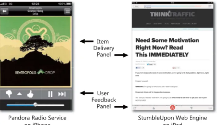
More recently, as a standalone Web service, Interactive Recommender Systems have emerged, by which 100% vol-ume of their services is comprised of direct user interactions with the recommender system over time. In many such sys-tems, there is no need for users to actively search for con-tent. Instead, items, such as webpages (StumbleUpon.com), songs (Pandora.com) or deals (Groupon.com), can be sequen-tially recommended to individual users, whilst feedback on recommended items is continuously observed. During the interactions, the recommender system is continuously re-fined by receiving feedback on delivered items and the user can enjoy sequential recommendations. Figure 1(a) provides snapshots of theStumbleUponWeb discovery service and the
Pandora radio streaming service. Such interactive recom-mendation services, despite easy to use, pose a ‘chicken-or-the-egg’ problem in providing accurate personalized recom-mendations. Successful personalized recommendation pre-diction requires adequate observations of user’s preferences. However, as illustrated in Figure 1(b), the preference ob-servation is restricted only to the items that have been rec-ommended. Therefore a critical problem is: how to rapidly learn a new user’s interest while not compromising his/her recommendation experience? Or, from the modelling per-spective, how to balance between the goals of learning the user profile and providing accurate predictions?
In such interactive recommendations, the first series of interactions with a new user are especially important. It is usually called the cold-start problem in the literature. Ex-isting techniques address the problem by using a two-phase process, i.e., to use active learning [21, 29] or an interview process (preference elicitation) [41, 16] to first learn the user profile, and then to make recommendations based on the established profile. The two-phase solution solves the prob-lem to a certain extent, but may not provide a complete solution. Asking the user to explicitly give ratings is still time-consuming and sometimes a burden for him/her; the user may have already left the service before his/her profile has been established. Recommendations would preferably be provided right from the very beginning and interests ac-quired by employing a less intrusive and implicit method of
6GTJUXG8GJOU9KX\OIK ;YKX ,KKJHGIQ 6GTKR UTO6NUTK UTO6GJ 9Z[SHRK;VUT=KH+TMOTK /ZKS *KRO\KX_ 6GTKR
(a) Two examples of Interactive Recommender Systems.
8KIUSSKTJKX 9_YZKS 8KIUSSKTJGZOUT
,KKJHGIQ ;YKX
(b) Non-stop Recommendation-feedback loop. Figure 1: Interactive Recommendation: a ‘chicken-or-the-egg’ problem. Recommendation requires feedback, whereas the feedback is only on the rec-ommended items. The scenario is also different from common relevance feedback in information retrieval, which normally handles the feedback in one or two iterations and lacks an established way to balance the exploration and exploitation [34].
gradually learning user profiles. A successful algorithm for interactive recommendation should not distinguish between the two phases, but continuously detect/learn the user pro-file while trying to satisfy the user at the same time.
The two inter-connected objectives mentioned above are closely related to the Exploitation-Exploration (EE) prob-lem [6, 15, 25]. It is the diprob-lemma whether, for each inter-action, we should try to satisfy the user’s interest with the best-guessed item based on current knowledge, or whether we should try some sub-optimal yet discriminative items to gain more knowledge about the user. The EE problem has been heavily studied in the machine learning and statis-tics communities, and multi-armed bandits are the generic setting of an EE problem. Many algorithms have been proposed under the independent-arm assumption, such as probability-based methods, e.g.,-greedy [6], epoch-greedy [24], Exp3 and Exp4 [7], and index-based methods, e.g., Git-tins Index [15] and the Upper-Confidence Bound [5, 6].
The EE principle has been applied for personalized con-tent recommendation. For example, in news article delivery tasks [25], a contextual-bandit algorithm has been proposed on the basis of the content features (texts) of the news ar-ticles and the browsing contexts of the users. The idea was to approximate the news articles’ profile features and max-imize the overall delivery performance across news articles using a linear prediction model.
However, it is unclear as to how to model the interaction in pure collaborative filtering settings where there is no content data to represent users and items and the only observations are ratings. In this paper, in order to naturally integrate with existing collaborative filtering approaches, we address
the Interactive Collaborative Filtering (ICF) problem under the popular matrix factorization framework, which has been proven to be effective in various recommendation competi-tions [22]. Specifically, we extend the probabilistic matrix factorization (PMF) [33] to build the probabilistic model of the user-item ratings over time. Our intention is to max-imize the users’ overall satisfaction throughout the recom-mendation journey. By modeling the rating with PMF, the uncertainty of a predicted rating comes from both the user feature vectors and the item feature vectors. While many existing multi-armed-bandit algorithms have addressed the problem by assuming arms to be independent [9, 24, 6], some others have tackled special cases where arms are structured in linear forms [5, 25]. In this paper, to consider the uncer-tainty in both the user and item feature vectors, we adopt empirical effective algorithms such as Thompson sampling [8] and construct a sampling process from their distribu-tions. Furthermore, in some cases, the item feature vectors are well-learnt and thus the item-side uncertainties could be disregarded. The problem then falls into a linear form in the item feature vectors, and thus various linear bandit al-gorithms [5] are applicable, including a variation of-greedy algorithm, linear and generalized linear upper-confidence-bound algorithms. Experimental results on both cold-start and warm-start (with drifting taste) users show significant improvements over several strong baselines for the Movie-Lens, EachMovie and Netflix datasets.
The rest of this paper is organized as follows. Section 2 discusses the related work. Our solution is formally pre-sented in Section 3. The experiment is described in Section 4, and we conclude this paper in Section 5.
2.
RELATED WORK
The CF research has been traditionally focused on pre-dicting the unknown ratings of a target user as accurately as possible from a collection of user profiles. Major solutions are categorized into two classes: The memory-based meth-ods make the recommendation by explicitly modelling the user or item similarities [19, 12] or combining them together [38], while the model-based methods provide recommenda-tions by developing a ‘model’ of user ratings. For instance, latent factor models have become quite popular during the recent years [20], while the matrix factorization techniques [22] have shown their effectiveness in various settings such as the Netflix and Yahoo! music competitions.
A key challenge in CF is to effectively predict preferences for new users, a problem generally referred to as the user cold-start problem [2, 35]. A straightforward method to tackle the problem is to interview the user to provide addi-tional information (e.g. favorite genres) or to ask the user to rate a set of items in order to provide enough data for the recommender system. The items used in the interview can be selected based on measures such as popularity, entropy and coverage [30, 31], or a decision tree to partition the users [41, 17]. Active learning is also deployed in order to identify the most informative set of training examples (items) with respect to some selection criterion, such as the expected in-formation gain [18, 21], with the target of minimizing the number of interactions. In summary, all those methods first explicitly figure out the user profile and then use the estab-lished user profile to make further recommendations. How-ever, asking users to take interviews is still time-consuming and sometimes a hurdle for them to overcome even if the effort has been kept minimum. By contrast, ICF that we propose does not distinguish between the stages of learn-ing user profiles and maklearn-ing satisfactory recommendations,
but naturally integrates them together. As such, any user, whether a new user or not, can immediately receive sequen-tial recommendations and explore items without overcoming the hassle of providing ratings before hand.
In the machine learning and statistics communities, the EE problem has been well studied by considering the multi-armed bandit settings [9, 24, 5]. Under the assumption that rewards of arms are independent to each other, -greedy is a straightforward algorithm that adds the probability of random exploration [6] into a greedy algorithm. The epoch-greedy method generalizes it for the case that the total time T is unknown so that the exploitation and exploration take place alternatively in each epoch to minimize the regret (i.e., the cumulative loss compared to the optimal one) [24], and it achieves a regret of O(Te 2/3) with a high probabil-ity. The confidence bound algorithms seek to find a region that bounds the expected payoff with a high probability, and within the region, the arm with highest upper confi-dence bound is selected: the EXP4 approach [7] achieves an
e
O(√T) regret with high probability. A drawback of these approaches lies in that when the number of arms is huge, ex-ploration becomes difficult. As such, the underlying struc-ture of the arms should be considered. A well-known sce-nario is that the expected reward is a linear function with respect to the features of them, where the linear bandit algo-rithm is proposed [5, 10, 1]. On the other hand, in the con-textual bandit model with side information, the structure is modelled by positioning each arm into a feature space [13], while a more general linear setting is discussed in [14]. Be-sides the above algorithms, Thompson sampling yet provides a more flexible way to tackle the multi-armed bandit prob-lems [8] which does not restrict the reward function forms to a linear one. Therefore, when we model the interaction, we propose to use Thompson sampling [8], which provides an empirical solution where the uncertainties of both the learnt feature vectors of the user and the item are considered.
The contextual bandit models have been applied to model news article recommendations [25] and online advertising [27], where in each timestep a context (in the form of a fea-ture vector) is revealed, and an arm (either a piece of news or an ad) is selected based on the context. The contextual bandit approaches can be naturally applied to both cases because in both cases the content features such as the user’s demography and location information, and the item’s tex-tual descriptions, preexist and can be immediately used to represent the ‘context’. In our domain-free scenario where users or items are presented only by ratings, it is, however, essential to derive a sensible representation for the corre-lated arms (items) and the contexts (users) and combine them together.
3.
ICF FRAMEWORK
3.1
Objective Function
Suppose the system hasN items andM users in record. The ratings between them are recorded in the preference ma-trixRM×Nin which each elementruiis the observed rating
from the useruto the itemi. Without loss of generality, we consider the following process in discrete timesteps. Sup-pose the target user is now denoted simply byu. At each timestept∈[1,2, . . . , T], the system delivers (recommends) an item to the target user. The user will then give feedback in the form of ratings, or ‘like’s and ‘dislike’s, or ignore the recommendation (‘unknown’s). In either way, we denote the feedback asru,i(t), the rating collected by the system from
useruto the recommended itemi(t) at timestept. In other words, ru,i(t) is the ‘reward’ collected by the system from
this target user. After receiving feedback, the system up-dates its model and decides which item to recommend next. Let’s denote H(t) as the available information at t the system has for the target user
H(t) ={i(1), ru,i(1), . . . , i(t−1), ru,i(t−1)}. (1) The item is selected according to a strategy π, which is defined as a function from the current information to the selected item:
i(t)≡π(H(t)). (2)
The optimal strategy should maximize the cumulated ex-pected reward duringT timesteps,
i∗(·) = arg max i(·) T X t=1 E[ru,i(t)], (3)
wherei(·) ={i(1), i(2), . . . , i(T)}. Because of the nature of recommender systems, here we use reward rather than regret to express the objective function, and maximizing cumula-tive reward is equivalent to minimizing regret. Here we con-sider the quality of recommendations at different timesteps as equally important, and summarize the user’s overall sat-isfaction at a given periodT. In our experiments, we show that a higher level of exploration is required in order to achieve a longer-term cumulative reward.
This objective falls into the target of the multi-armed ban-dit problem, where we regard each item as each arm of the bandit. The next questions are how to estimate the reward and how to optimize the objective function. Using the la-tent factor model [20], the rating is a product of user and item feature vectorspuandqi. This is widely used in many
CF algorithms:
ru,i=p0uqi+η, (4)
whereη∼ N(0, σ2) is the observation noise. The objective function is then re-formulated as follows:
i∗(·) = arg max i(·) T X t=1 E[ru,i(t)|t] = arg max i(·) T X t=1 Epu,qi(t)[p 0 uqi(t)|t]. (5) The question now is how to optimize the objective function.
3.2
Item Selection via Sampling
Both pu and qi are random variables following certain
distributionp(pu,qi|t). A heuristic solution of Eq. (5) is to samplean item based on its probability of being optimal [8],
p(i(t) =i) = Z I E(rui|pu,qi) = max j E(ruj|pu,qj) · p(pu,qi|t)dqidpu, (6)
where I is the indicator function; it is 1 when the
equal-ity holds (i.e., when itemihas the highest expected rating givenpu andqi); otherwise 0. Thus, integratingpuandqi
out gives the probability of being optimal at t for item i. The integration is computational expensive, but in practice, no need to compute it explicitly. In this paper, a sampling approach, called Thompson sampling, is leveraged to ap-proximate the integration in Eq. (6) [8]. A nice property of Thompson sampling is that the integration is circumvented by sampling both the user and item feature vectors together from their distributions (consider the uncertainty from both
aspects) and picking the item that leads to the largest ex-pectation of the reward:
i∗(t)ts= arg max i E
(rui|p˜u,q˜i), (7)
where p˜u and q˜i mean the sampled user and item feature
vectors, which will be described in the next section.
3.2.1
Distributions of User and Item Feature Vectors
In this section, we adopt the PMF model [33] to build the distributions for the user and the item feature vectors, which are then used to generate the samples. Specifically, the con-ditional probability distribution of the rating given the user and item feature vectors follows a Gaussian distribution
p(rui|p0uqi, σ2) =N(rui|p0uqi, σ2). (8)
We denoteP (Q) as the user (item) feature vector ma-trix, where each row vector represents a user (item) feature vector (P = [p1,p2, . . . ,pM]0, Q= [q1,q2, . . . ,qN]0). The
distribution of the preference matrix R given P and Q is then the joint probability, i.e.,
p(R|P, Q, σ2) = M Y u=1 N Y i=1 [N(rui|p0uqi, σ2)]δui, (9)
whereδij= 1 if userurated itemiandδij= 0 otherwise.
Similar to the PMF model [33], we define the prior dis-tributions of the user and item feature vectors as Gaussian with prior variancesσ2pandσ2q
p(pu|σp2) =N(pu|0, σ2pI), (10)
p(qi|σ2q) =N(qi|0, σq2I). (11)
By observing the ratingsR, we can obtain the posterior distributions for the user and item feature vectors [33]. Here we focus on the conditional distribution of the user (item) feature vectors, given the current item (user) feature vec-tors to implement Markov chain Monte Carlo and Gibbs Sampling (MCMC-Gibbs): p(P|R, Q, σ2, σp2, σ 2 q)∝p(R|P, Q, σ 2 )·p(P|σ2p, σ 2 q) ∝ M Y u=1 N(pu|0, σ2pI) N Y i=1 [N(rui|p 0 uqi, σ2)]δui ∝ M Y u=1 exp − 1 2σ2 σ2 σ2 p p0upu+ X δui=1 (rui−p0uqi)2 ∝ M Y u=1 exp − 1 2σ2 p0u( X δui=1 qiq 0 i+ σ2 σ2 p I)pu−2 X δui=1 ruiq 0 ipu ∝ M Y u=1 N(pu|µu,Σu). (12)
It means for each user its feature vector follows a Gaussian distribution given item feature vectors:
p(pu|R,Q, σ2, σp2, σq2) =N(pu|µu,Σu), (13)
µu= (D0uDu+λpI)−1Du0ru, (14)
Σu= (D0uDu+λpI)−1σ2 . (15)
Here, Du is the observational matrix for the user, each
row of which is the feature vectors of the user rated items sampled from their posteriors. rudenotes the vector of
cor-responding ratings of these items for the given useru, and λp=σ2/σ2p.
Algorithm 1Thompson sampling
Require: parameters for the item feature vector distribu-tions Θ ={(ν1,Ψ1), . . . ,(νN,ΨN)},σ,λp Initialization: A←λpI b←0 fort= 1,2,3, ..., T do Estimateµu,t=A−1b Estimate Σu,t=A−1σ2
Sample ˜pu,t fromN(pu,t|µu,t,Σu,t)
Sample ˜qi fromN(qi|νi,Ψi)for{i∈ {1,2, . . . , N}}
Select the armi∗(t) = arg maxip˜
0
uq˜i
Receive the rewardru,i∗(t) UpdateA←A+ ˜qi∗(t)q˜0
i∗(t) Updateb←b+ru,i∗(t)q˜i∗(t)
end for
Similarly, the posterior distribution for the item feature vector qi conditioned on the sampled user feature vectors
can be obtained as p(qi|R,P, σ2, σp2, σ 2 q) =N(qi|νi,Ψi), (16) νi= (B0iBi+λqI)−1B0iri, (17) Ψi= (B 0 iBi+λqI) −1 σ2, (18)
andBiis the observational matrix with each row the
sam-pled user feature vector.
The distributions converge by alternatively sampling the item and the user feature vectors according to the condi-tional distributions for them. Then both the expected user and item feature vectors (µuandνi) and their uncertainties
(Σuand Ψi) are obtained.
3.2.2
Combing Thompson Sampling with PMF
Thompson sampling can be implemented according to the distributions while they are updated online whenever new ratings are collected by the system. However, in the ICF scenario, the distribution of the target user’s feature vec-tor is much more sensitive to his/her feedback on the items. On the item side, since each item has usually collected rel-atively sufficient ratings, it is not necessary to retrain its feature vector immediately after receiving each rating from the target user, and we choose to periodically retrain them. Therefore, we simply use the notation q˜i to express
sam-pled item feature vector from the presently calculated item feature vector distribution. For the target user, its observa-tional matrix grows each time, and its distribution can be described similarly conditioned on the observations:
˜
pu,t∼ N(pu,t|µu,t,Σu,t), (19)
where µu,t= (D 0 u,tDu,t+λpI) −1 Du,t0 ru,t, (20) Σu,t= (D 0 u,tDu,t+λpI) −1 σ2. (21)
Similarly,Du,t is the observational matrix with each row
is the recommended item feature vector, and Σu,t is the
uncertainty of the user feature vector at timet.
From Eq. (7), the Thompson sampling method with the PMF modeling suggests to choose the item with the highest value of the inner product of the sampled values, and Eq. (7) can be approximated as:
i∗(t)ts= arg max i
˜
p0u,tq˜i, (22)
where ˜pu,tis sampled from the estimated distribution in Eq.
(19). The algorithm is described in Algorithm 1.
Thompson sampling enables exploration through the ‘width’ of the distributions of the inner product of the user and
Algorithm 2Linear UCB
Require: MAP solution of item feature vectors Q =
{ν1, . . . ,νN},σ,λp, andα∈R+ Initialization: A←λpI b←0 fort= 1,2,3, ..., T do Estimateµu,t=A−1b Estimate Σu,t=A−1σ2
Choose the item i∗(t) = arg max
i
µ0u,tνi+α||νi||2,Σu,t
Receive the rewardru,i∗(t) UpdateA←A+νi∗(t)νi0∗(t) Updateb←b+ru,i∗(t)νi∗(t)
end for
item feature vectors. The ‘width’ further comes from both the uncertainties of the user and item feature vectors. By this approach described above, the uncertainties of the user and item feature vectors are considered on the same foot-ing. However, considering ICF as a user-centric scenario (Figure 1), the obtained knowledge on the target user side may be much more important than that on the item side, especially when items have collected many ratings and thus are always already well-learnt. Therefore, in the following part, we adopt a biased view so that the item feature vectors are assumed to be well-learnt as the maximum a posterior (MAP) solutionνifrom the distributions obtained by PMF,
and only the user feature vector distributions are maintained for the sampling process.
3.3
Item Selection via Confidence Bound
With the item feature vectors known and fixed, the re-ward in Eq. (4) tends to be a linear form with the item feature vectors as coefficients, and the essence of the EE is to approach the user feature vector. Therefore, such prob-lem falls into the framework of linear bandits [5]. Linear Upper-Confidence-Bound (UCB) algorithm, and its varia-tions are widely used for such problems. In this way, we take the MAP estimation of the item feature vectorsνi as
the representatives of the items and assume them to be fixed. In the following, linear and generalized linear UCB algo-rithms are presented for our problem respectively. A varia-tion of-greedy algorithm is also provided for comparison.
3.3.1
Linear UCB
As mentioned above, assuming the item feature vectors as fixed, the reward function reduces to be linear in the item feature vectors, and the objective function in Eq. (4) is further written as i∗(·) = arg max i(·) T X t=1
E[ru,i(t)] = arg max i(·) T X t=1 Epu[p 0 u|t]νi(t), (23) whereEpu[p 0
u|t] can be estimated according to Eq. (20).
The expected user feature vector can be obtained accord-ing to Eq. (20). Now the uncertainty of the reward can be obtained as the estimated variance of the inner product of the user and item feature vectors p0uνi, which comes from
the uncertainty of the estimation in the user feature vector. The estimated variance is the 2-norm based on Σu,t
(accord-ing to Eq. (21), but note that here the observational matrix is made up of the posterior feature vectors of the items):
||νi||2,Σu,t≡ p
ν0
iΣu,tνi. (24)
Algorithm 3GLM-UCB
Require: MAP solution of item feature vectors Q =
{ν1, . . . ,νN},σ,λp, andc∈R+ Initialization: A←λpI
fort= 1,2,3, . . . , T do Estimate ˆpu,t by Eq. (29)
Estimate Σu,t=A−1σ2
Choose the item i∗(t) = arg max i ρ( ˆp0u,tνi) +c p logt||νi||2,Σu,t
Receive the rewardru,i∗(t) UpdateA←A+νi∗(t)νi0∗(t)
end for
Algorithm 4Linear-greedy
Require: MAP solution of item feature vectors Q =
{ν1, . . . ,νN},λpand∈[0,1]
Initialization: A←λpI
b←0
fort= 1,2,3, ..., T do Estimateµu,t=A−1b
With probability 1−choose the item i∗(t) = arg max
i µ
0
u,tνi
Otherwise choose an item randomly Receive the rewardru,i∗(t)
UpdateA←A+νi∗(t)νi0∗(t) Updateb←b+ru,i∗(t)νi∗(t)
end for
According to [37], with the item feature vectors known and fixed, the expectation of the reward by choosing itemi is bounded in the interval Θi,twith probability at least 1−ζ
Θi,t= µ0u,tνi−α||νi||2,Σu,t,µ 0 u,tνi+α||νi||2,Σu,t (25) whereα= 1+pln (2/ζ)/2. The bounded interval motivates an UCB bandit algorithm, i.e., at each timestep, choose the item with the highest upper confidence bound:
i∗(t)l= arg max i
µ0u,tνi+α||νi||2,Σu,t
. (26)
The algorithm is given in Algorithm 2. The algorithm is proven to have a very tight regret bound of ˜O(√T) [25].
As defined in Eq. (21), matrix Σu,t is a regularized fisher
information matrix, measuring how much ‘information’ is known about the user feature vector from the previously rec-ommended items, given the item feature vectors are known already. That is, to recommend an item that maximizes
||νi||2,Σu,t is to recommend an item that has been the least represented (understood) by the perviously recommended items.
3.3.2
Generalized Linear UCB
The problem can be also linked to the generalized lin-ear bandit problem in [14], which gives a general solution Generalized Linear Model Bandit-Upper Confidence Bound (GLM-UCB) if we assume the reward takes the following form ru,i(t)=ρ p 0 uqi(t) +η(t), (27)
whereρis a monotonically increasing function which takes a linear or nonlinear form. Here we give two options of functionρ, a linear form suggested in Eq. (4), and a sigmoid
form
ρ(p0uqi) =
1
1 +e−pu0qi. (28) Similar to the derivations in LinUCB, here the item fea-ture vectors qi are approximated by the maximum a
pos-terior (MAP) solution νi. On the other hand, we need to
estimate the user feature vector according to the generalized linear model, which here we denote as ˆpu,t (note that here
the solution ˆpu,t is no longer the MAP solution in Eq. (20)
due to the nonlinear functionρ). In general, according to [14], the quasi-likelihood estimator ˆpu,t of Eq. (27) is the
solution of t−1 X τ=1 ru,i(τ)−ρ( ˆp 0 u,tνi(τ)) νi(τ)= 0. (29)
Specifically, for a sigmoid form, it is estimated as
t−1 X τ=1 ru,i(τ)− 1 1 +e−pˆ0u,tνi(τ) νi(τ)= 0. (30)
For a linear form, the estimate is the same as the max-imum posterior estimation of the user feature vectors Eq. (20).
The GLM-UCB algorithm follows a similar process as Lin-ear UCB, i.e., firstly ˆpu,tis estimated, and the choice of the
item is based on the estimated ˆpu,tbut with exploration part
added which is 2-norm based on Σu,t (Eq. (24)) multiplied
by a factorc√logt[14] i∗(t)gl= arg max i ρ( ˆp0u,tνi) +c p logt||νi||2,Σu,t . (31)
The GLM-UCB algorithm is illustrated in Algorithm 3. Note that exploration termαis time-dependent:
α=α(t) =cplogt, (32)
where c is a constant with respect to t [14]. With term c√logt, the decreasing trend of||νi||2,Σu,t is weakened so that the exploration level is maintained to some extent. Us-ing the conclusion from [14], GLM-UCB has a regret bound of ˜O(√T).1
Just like the other index-based EE algorithms [5], the algorithms have a low computational complexity, which is O(T3+K2N).
3.3.3
Linear
-greedy
The linear-greedy algorithm is based on the greedy strat-egy under our setting, which can be described as
i∗(t)g= arg max i
µ0u,tνi. (33)
Becauseµu,tandνican be seen as the MAP solutions for
the PMF model, which can also be referred as the solutions by singular vector decomposition (SVD). We refer to the greedy strategy as greedy SVD, or simply SVD.
The greedy strategy is the myopic strategy that always picks the item leading to the highest expected reward based on current knowledge. Linear -greedy we adopt here is the naive algorithm which chooses the greedy strategy with probability 1−and explores into random items with prob-ability. The algorithm is described in Algorithm 4.
For the above algorithms, two factors contribute to the selection of the item: the exploitation factor suggested by the greedy algorithm Eq. (33), and the exploration factor 1The detailed form of the bound is looser than that of Lin-UCB but it is more general.
Table 1: Characteristics of the datasets.
Dataset MovieLens EachMovie Netflix
#users 943 72,916 480,189
#items 1,683 1,648 17,770
#ratings per user 106.04 38.56 209.25
#ratings per item 59.42 1706.30 5654.50
total #ratings 100,000 2,811,983 100,480,507
which is controlled by parametersα,candrespectively. For each of the three algorithms, the larger the parameter is, the more emphasis is put onto the exploration effort accordingly.
4.
EXPERIMENTS
Experiments are carefully designed to answer the follow-ing questions: (1) How can EE algorithms outperform my-opic CF algorithms for the cold-start users? (2) Among the EE algorithms, which one is the most effective and why? (3) Are the algorithms also effective for warm-start users, espe-cially those whose interests change over time? (4) Consid-ering top-nrecommendation over time, can the algorithms still be effective?
4.1
Datasets
We base our experiments on three popular datasets Movie-Lens (100k), EachMovie and Netflix. The basic information of the datasets is summarized in Table 1.
Due to the interactive nature of our problem, an online ex-periment with true interactions from users would be ideal, but it is not always possible [25]. Instead, we follow an unbiased offline evaluation scheme for contextubandit al-gorithms in [26]. In our setting, we assume that the ratings recorded in the datasets are users’ instinctive actions, not biased by the recommendations provided by the system. In this way, the records can be treated as unbiased to represent the feedback in an interactive setting [41].
We normalize the ratings into the range [−1,1] and split the data into two user-disjoint sets: the training users and their ratings are used to train the parameters for the item distributions, as required in Thompson Sampling, and to obtain the MAP solutions of the item feature vectors, as re-quired in UCB-based algorithms (Section 3.2.1). The item feature vector information is maintained as unchanged dur-ing the test phase when the test users go through the inter-active recommendation process duringT timesteps because the collected ratings from the target user have trivial ef-fect on the item feature vector distributions. According to the purpose (whether to test the performance on cold-start users, or on warm-start users), we select test users based on different criteria, detailed in each subsection.
4.2
Compared Algorithms
The baselines include:
Random. In each interaction, randomly chooses an item from the entire item set to recommend to the target user.
Popularity-based (Pop). The system picks the most popular items to recommend to the target user.
Greedy SVD (SVD).This algorithm is built upon the SVD approach. We regard it as the myopic algorithm in ICF. For each target user, the system needs to retrain the SVD model after each interaction.
Active Learning (AL). Active learning methods have been proposed for the cold-start problem [18]. The idea is to minimize the uncertainty in the model, so that the item with highest uncertainty is selected [32].
Interview Process (Interview). The interview pro-cess first constructs the user profile with a number of most discriminative items, and then shifts to the greedy
recom-Table 2: Cold-start performance on MovieLens, EachMovie, and Netflix dataset.
Dataset MovieLens (100k) EachMovie Netflix
Measure Cumulative Precision Cumulative Precision Cumulative Precision
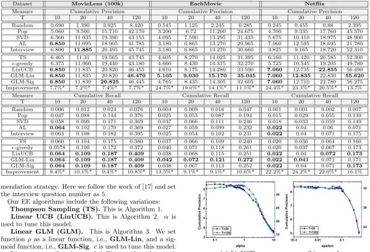
T 10 20 40 120 10 20 40 120 10 20 40 120 Random 0.690 1.390 2.925 8.420 0.545 1.125 2.245 6.285 0.245 0.455 0.88 2.395 Pop 5.060 9.500 15.710 42.170 3.200 6.72 11.200 24.675 4.700 9.335 17.760 45.370 SVD 6.360 11.035 19.390 43.155 4.095 7.590 13.295 31.435 5.675 10.410 18.975 48.900 AL 6.850 11.095 18.905 41.785 3.180 6.865 13.270 29.965 7.060 12.595 18.695 21.780 Interview 6.800 11.885 20.495 45.745 3.180 6.865 13.270 30.660 3.825 9.165 18.720 52.310 TS 6.465 11.31 19.565 43.745 4.605 8.270 14.025 31.395 6.160 11.420 20.585 52.300 -greedy 6.375 11.060 19.440 43.180 4.660 8.430 14.315 32.270 5.725 10.545 19.205 49.780 LinUCB 6.850 11.835 20.820 46.455 4.610 8.175 14.280 33.590 7.060 12.735 22.855 56.490 GLM-Lin 6.850 11.835 20.820 46.470 5.105 9.030 15.170 35.045 7.060 12.835 22.830 55.620 GLM-Sig 6.850 11.830 20.825 46.445 4.765 8.435 14.305 32.605 7.060 12.710 22.780 56.275 Improvement 7.7%* 7.2%* 7.4%* 7.7%* 24.7%* 19.0%* 14.1%* 11.5%* 24.4%* 23.3%* 20.5%* 13.7%
Measure Cumulative Recall Cumulative Recall Cumulative Recall
T 10 20 40 120 10 20 40 120 10 20 40 120 Random 0.006 0.012 0.024 0.076 0.004 0.009 0.016 0.047 0.001 0.001 0.002 0.007 Pop 0.047 0.088 0.144 0.376 0.025 0.053 0.087 0.194 0.015 0.029 0.055 0.139 SVD 0.058 0.099 0.171 0.369 0.037 0.066 0.111 0.246 0.018 0.033 0.059 0.149 AL 0.064 0.102 0.170 0.369 0.027 0.059 0.099 0.232 0.022 0.04 0.06 0.071 Interview 0.063 0.108 0.182 0.395 0.025 0.054 0.102 0.231 0.022 0.04 0.071 0.175 TS 0.060 0.104 0.175 0.380 0.037 0.066 0.109 0.240 0.020 0.036 0.064 0.160 -greedy 0.0578 0.100 0.172 0.372 0.040 0.071 0.118 0.261 0.020 0.037 0.067 0.173 LinUCB 0.064 0.109 0.187 0.409 0.038 0.068 0.115 0.251 0.022 0.04 0.072 0.173 GLM-Lin 0.064 0.109 0.187 0.409 0.042 0.072 0.121 0.272 0.022 0.041 0.071 0.171 GLM-Sig 0.064 0.109 0.187 0.409 0.038 0.067 0.113 0.252 0.022 0.04 0.071 0.173 Improvement 9.4%* 10.1%* 9.4%* 10.8%* 13.5%* 9.1%* 9.1%* 10.6%* 22.2%* 24.2%* 22.0%* 16.1%
mendation strategy. Here we follow the work of [17] and set the interview question number as 5.
Our EE algorithms include the following variations: Thompson Sampling (TS).This is Algorithm 1.
Linear UCB (LinUCB). This is Algorithm 2. α is used to tune this model.
Linear GLM (GLM). This is Algorithm 3. We set function ρ as a linear function, i.e.,GLM-Lin, and a sig-moid function, i.e.,GLM-Sig.cis used to tune this model. Linear -greedy. (-greedy)This is Algorithm 4. A tuning parameteris used to control the balance between the exploitation and exploration.
In addition, we add a constraint for all the algorithms that the same item should not be repeatedly recommended as suggested in most previous ranking-oriented recommen-dation settings [28, 40].
4.3
Evaluation Measures
Three evaluation metrics are used:
Cumulative Precision@T. A straightforward evalua-tion measure is the number of the positive ratings collected during the totalT interactions:
precision@T = 1 #users X users T X t=1 θhit. (34)
For both datasets, we defineθhit= 1 if the rating is no less than 4, and 0 otherwise, similar to the definition of positive ratings in previous work [3].
Cumulative Recall@T. We can also check for the recall duringT timesteps of the interactions.
recall@T = 1 #users X users T X t=1 θhit #preferences . (35) Cumulative nDCG@n. For the case that multiple items are shown in one interaction, the ranking of the item listed is also important: it is more useful to have the highly rel-evant items appear earlier in the ranking list. We use the normalized discounted cumulative gain (nDCG@n) as the
0.1 1 10 3 4 5 6 7 8 T=20 T=120 alpha C um ul at iv e Pr ec is io n 15 20 25 30 (a) LinUCB 1E-3 0.01 0.1 5 6 7 8 T=20 T=120) epsilon C um ul at iv e Pr ec is io n 24 28 32 (b)-greedy
Figure 2: Cumulative precision against parameter turning on EachMovie. ranking measure nDCG@n= 1 Z n X j=1 2rj−1 log2(j+ 1) , (36)
whererjis the real rating of the item shown at ranking
posi-tionj. Zis the normalization factor making the score of the optimal ranking to 1 such that 0≤nDCG@n≤1. Similar to the cumulative precision and recall, here the cumulative nDCG@nshould also take sum overT and average on users.
4.4
Cold-start Cases
4.4.1
Test User Selection
In order to test the system’s performance on cold-start users, we first select users with sufficient numbers of recorded ratings in order to test the performance. Here we randomly select 200 users with more than 120 ratings because up to T = 120 interactions are studied. Then the parameters of item feature vector distributions are trained without these user’s ratings according to Section 3.2.1.
4.4.2
Performance Comparison
Performances of proposed algorithms and the baselines for cold-start users are compared and summarized in Table 2. Optimally tuned parameters have been adopted for each T = 10,20,40,80,120. The effect of parameters will be dis-cussed in Section 4.4.3. The best-performing algorithm is
Table 3: Performance on Warm-start Users with Taste Drift on MovieLens and EachMovie.
Dataset MovieLens (100k) EachMovie
Measure Cumulative Precision Cumulative Precision
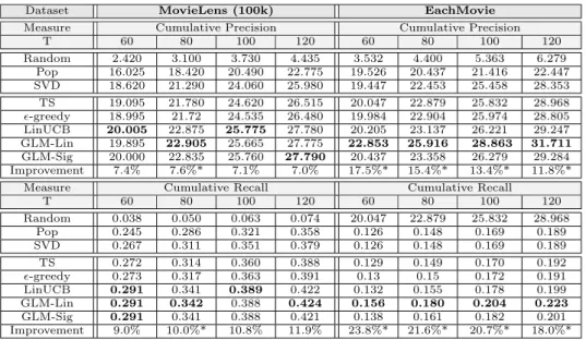
T 60 80 100 120 60 80 100 120 Random 2.420 3.100 3.730 4.435 3.532 4.400 5.363 6.279 Pop 16.025 18.420 20.490 22.775 19.526 20.437 21.416 22.447 SVD 18.620 21.290 24.060 25.980 19.447 22.453 25.458 28.353 TS 19.095 21.780 24.620 26.515 20.047 22.879 25.832 28.968 -greedy 18.995 21.72 24.535 26.480 19.984 22.904 25.974 28.805 LinUCB 20.005 22.875 25.775 27.780 20.205 23.137 26.221 29.247 GLM-Lin 19.895 22.905 25.665 27.775 22.853 25.916 28.863 31.711 GLM-Sig 20.000 22.835 25.760 27.790 20.437 23.358 26.279 29.284 Improvement 7.4% 7.6%* 7.1% 7.0% 17.5%* 15.4%* 13.4%* 11.8%*
Measure Cumulative Recall Cumulative Recall
T 60 80 100 120 60 80 100 120 Random 0.038 0.050 0.063 0.074 20.047 22.879 25.832 28.968 Pop 0.245 0.286 0.321 0.358 0.126 0.148 0.169 0.189 SVD 0.267 0.311 0.351 0.379 0.126 0.148 0.169 0.189 TS 0.272 0.314 0.360 0.388 0.129 0.149 0.170 0.192 -greedy 0.273 0.317 0.363 0.391 0.13 0.15 0.172 0.191 LinUCB 0.291 0.341 0.389 0.422 0.132 0.155 0.178 0.199 GLM-Lin 0.291 0.342 0.388 0.424 0.156 0.180 0.204 0.223 GLM-Sig 0.291 0.341 0.388 0.421 0.138 0.161 0.182 0.201 Improvement 9.0% 10.0%* 10.8% 11.9% 23.8%* 21.6%* 20.7%* 18.0%*
shown in boldface with∗marking significant improvements (by Wilcoxon signed-rank test). The row of improvement shows the increases brought by the best-performing algo-rithm compared to the greedy SVD strategy.
The observations can be summarized into the following points: (1) The Thompson sampling algorithm generally works better than the greedy SVD, or the -greedy algo-rithm. In most cases, Thompson sampling also exceeds other baseline algorithms (according to the cumulative precision). It means that the exploration by considering the uncertain-ties of the user and items according to their probability dis-tributions, is more promising than randomly conducting ex-plorations. Nevertheless, the Thompson sampling fails to outperform the LinUCB or GLM algorithms. (2) In almost all cases, the UCB-based algorithms perform better than the baselines. In MovieLens and Netflix, the three UCB-based algorithms have close performances while in Each-Movie GLM-Lin outperforms all the baselines. The increase by the proposed EE algorithm compared to SVD is up to 7.7% on MovieLens, 24.7% on Eachmovie, and 24.4% on Netflix (according to the cumulative precision). All of the improvements (except one) are statistically significant. (3) Among all the proposed EE algorithms, linear-greedy per-forms worst, but still better than the greedy SVD. It sug-gests that adding some level of exploration can always im-prove the pure exploitation strategy. (4) The greedy SVD outperforms the popularity-based strategy, and obviously the random strategy performs the worst. (5) The interview strategy performs better than the active learning strategy in the long run, because it shifts to exploitation after learn-ing the user by exploration (5 timesteps). For all the three datasets, however, the interview strategy is not as good as the algorithms which are proposed based on ICF framework. There are two possible reasons that UCB-based algorithms outperform the Thompson sampling method. First, the user uncertainties may play a much more important role in the ICF scenario. Consideration on item-side uncertainties may be helpful for learning the item feature vectors in the long run, but in this user-centric system, it may hamper the user experience. Second, compared with the UCB-based algo-rithms which explicitly pursue the highest possible perfor-mance for each item as their exploration strategy, Thomp-son sampling involves considerations on both the positive and negative possible performances for each item. In
ad-dition, the sampling process itself imports the exploration instability. However, the UCB-based algorithms are built on the assumption that the item feature vectors are well-learnt. In the case of very limited available data and thus underestimated item feature vectors, it may be necessary to consider the uncertainty of item feature vectors. We leave this problem as our future work.
4.4.3
Impact of Trade-off Parameters
The algorithm-dependent parameters α,c, are used to balance between the exploitation and exploration. Here we focus on the cumulative precision as the measure of the per-formance, and investigate how the performance depends on the parameters, with respect to two horizons T = 20 and T = 120, shown in Figure 2.2 We only show the impact ofα for LinUCB andfor linear-greedy due to the page limit whereas other cases display the similar trends.
We observe that when either αor (for either the case ofT = 20 or T = 120) increases, the performance first in-creases, and then falls down. The peak performance corre-sponds to the optimal parameter which forT = 20 is smaller than that for T = 120. This is intuitively correct because more exploration is needed when a longer-term satisfaction is targeted. In practice, for the decision ofT, we can make use of the statistics from the system record, such as the average life-time of the users.
4.5
Warm-start Cases with Taste Drift
4.5.1
Test User Selection
Through this experiment, we aim to answer the question whether the algorithms are also applicable on warm-start users to follow up their interests throughout the interac-tions, especially when their tastes are changing over time. To do this, we first divide the rating records of the users (whose ratings are more than 120) into two periods (set 1 and set 2). Then, we employ the genre information of the items as an indication of the user interest [36]. That is, we calculate the cosine similarity between the genre vectors of the two periods. We choose the users with the smallest cosine similarity as an indication that they have significant interest drift across the two time periods. All the other users 2Empirically, we do not necessarily restrict αaccording to Eq. (25).
Table 4: Performance for Multiple-item Recommendations by Cumulative nDCG.
Dataset MovieLens EachMovie Netflix
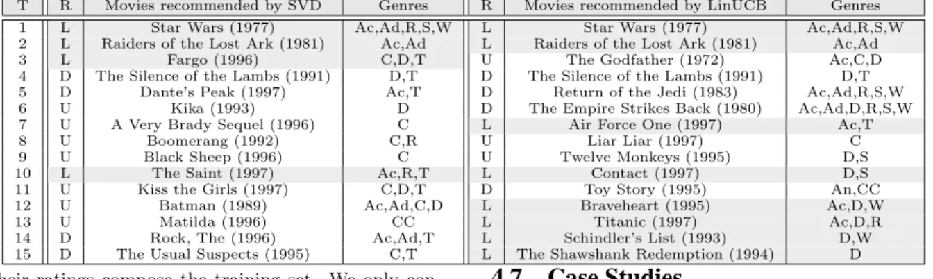
Measure nDCG@3 nDCG@5 nDCG@3 nDCG@5 nDCG@3 nDCG@5 T 20 40 10 20 20 40 10 20 20 40 10 20 Random 0.750 1.563 0.369 0.701 0.619 1.280 0.290 0.586 0.263 0.46 0.145 0.255 Pop 4.876 8.669 2.666 4.633 3.864 5.588 1.752 2.913 5.29 9.165 2.687 4.693 SVD 6.099 9.832 3.361 5.345 5.043 8.083 2.651 4.379 7.465 12.733 3.983 6.837 TS 6.195 9.912 3.393 5.452 5.167 8.320 2.678 4.431 7.962 13.887 4.237 7.363 -greedy 6.080 9.845 3.352 5.333 5.181 8.482 2.689 4.509 7.591 13.009 4.006 6.87 LinUCB 6.391 10.250 3.419 5.519 4.996 8.381 2.689 4.466 8.113 14.085 4.221 7.376 GLM-Lin 6.369 10.253 3.427 5.472 5.367 8.862 2.815 4.719 7.834 13.569 4.145 7.265 GLM-Sig 6.363 10.236 3.424 5.432 5.156 8.375 2.718 4.494 8.081 14.094 4.199 7.353 Improvement 4.8% 4.3% 2.0%* 3.3%* 6.4% 9.6% 6.2%* 7.7%* 8.7%* 10.7%* 6.4%* 7.9%*
Table 5: A case study of cold-start user #454 on Movielens. User feedback R: L-Like, D-Dislike, U-Unknown. Movie Genre Abbreviation: Ac-Action, Ad-Adventure, An-Animation, C-Comedy, CC-Children’s Comedy, D-Drama, R-Romance, S-Scientific Fiction, T-Thriller, W-War.
T R Movies recommended by SVD Genres R Movies recommended by LinUCB Genres
1 L Star Wars (1977) Ac,Ad,R,S,W L Star Wars (1977) Ac,Ad,R,S,W
2 L Raiders of the Lost Ark (1981) Ac,Ad L Raiders of the Lost Ark (1981) Ac,Ad
3 L Fargo (1996) C,D,T U The Godfather (1972) Ac,C,D
4 D The Silence of the Lambs (1991) D,T D The Silence of the Lambs (1991) D,T
5 D Dante’s Peak (1997) Ac,T D Return of the Jedi (1983) Ac,Ad,R,S,W
6 U Kika (1993) D D The Empire Strikes Back (1980) Ac,Ad,D,R,S,W
7 U A Very Brady Sequel (1996) C L Air Force One (1997) Ac,T
8 U Boomerang (1992) C,R U Liar Liar (1997) C
9 U Black Sheep (1996) C U Twelve Monkeys (1995) D,S
10 L The Saint (1997) Ac,R,T L Contact (1997) D,S
11 U Kiss the Girls (1997) C,D,T D Toy Story (1995) An,CC
12 U Batman (1989) Ac,Ad,C,D L Braveheart (1995) Ac,D,W
13 U Matilda (1996) CC L Titanic (1997) Ac,D,R
14 D Rock, The (1996) Ac,Ad,T L Schindler’s List (1993) D,W
15 D The Usual Suspects (1995) C,T L The Shawshank Redemption (1994) D
with their ratings compose the training set. We only con-duct experiments on MovieLens and EachMovie datasets, as there is no movie genre information for Netflix dataset.
4.5.2
Adaptability to Taste Drift
In order to test how the system can catch the users’ taste drift, we conduct the empirical experiment as follows: for each user, in the first period with 60 interactions, we use set 1 as the ground truth of the test users; and then, from the 61st interaction, the ground truth is changed from set 1 to set 2 to simulate the process of his/her taste drift. Table 3 presents the results of our proposed algorithms compared to the baselines on the datasets, respectively. Because we focus on the performance when the user has changed the interest, only the results forT ≥60 are shown.
From the results, it can be seen that the proposed al-gorithms outperform the baselines for both datasets. When compared with the greedy SVD method, the improvement is up to 7.6% on MovieLens dataset, and 17.5% on EachMovie dataset. Among the algorithms, the UCB-based algorithms perform better than Thompson sampling method, which is similar to the results for the cold-start experiments.
4.6
Top-
NRanking Performance
We also conduct an experiment with multiple item slots at each interaction. The ranking-aware measure nDCG is used to test the performance. The test users are the same as the ones in the cold-start setting. The only difference is that the number of interactions is reduced since the number of recommended items in each interaction increases. The results are shown in Table 4.
A similar trend is shown compared to the case of one item at each timestep: on MovieLens, either LinUCB or GLM-Lin performs the best, and on EachMovie, GLM-GLM-Lin always performs best. The results indicate that the algorithms still outperform the baselines in the multiple item setting. In addition, the performance on nDCG measure suggests that our proposed algorithms are also capable of the CF ranking problems.
4.7
Case Studies
In order to better illustrate why the algorithms outper-form greedy SVD, we present two case studies for a cold-start user and a taste-drift user respectively.
4.7.1
A Cold-start User Case
In Table 5, we present the first 15 sequentially recom-mended movies to a typical user #454 on Movielens by greedy SVD and LinUCB, and the corresponding feedback. From the results we can see that (i) LinUCB earns more ‘like’ feedback and less ‘dislike’ and ‘unknown’ feedback; (ii) After the first three ‘likes’, SVD keeps recommending ac-tion, crime and thriller movies, which is somewhat myopic; (iii) For LinUCB, after receiving the positive and negative feedback on action, war, thriller, and science fiction movies, it tries different genres such as drama, comedy and anima-tion. After the next five interactions, LinUCB discovers the other interest in drama movies.
4.7.2
A Warm-start User with Taste Drift
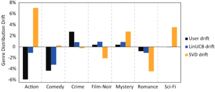
In Figure 3, we show a typical taste-drift case of user #833 on Movielens. Specifically, 7 typical movie genres (out of 18) are involved here. The black bars show the user’s taste drift by calculating the percentage difference of the normalized distributions on each genre between two time periods as in Section 4.5.1. The blue and orange bars show the percent-age difference on each genre of the recommended items by LinUCB and greedy SVD respectively. We see that LinUCB captures the user’s taste drift in a better way than greedy SVD: (i) For these genres, LinUCB captures the drift di-rection. For example, the user’s interest in Comedy movies decreases (-4.3%3) between the two periods. LinUCB also recommends fewer (-3.2%) Action movies but greedy SVD recommends more (+1.1%) Action movies to the user. (ii) For most genres, LinUCB to some extent captures the drift degree, e.g., the user has a 0.8% interest decrease on Ro-3The percentage measures the difference of the proportion of Comedy movies the user watches between the two periods.
-6% -4% -2% 0 2% 4% 6% 8%
Ac on Comedy Crime Film-Noir Mystery Romance Sci-Fi
User dri LinUCB dri SVD dri
Figure 3: A case study on handling taste drift. mance movies and LinUCB also recommend 1.1% fewer Ro-mance movies, but greedy SVD dramatically decreases this type of movies to the extent of 4.4%.
5.
CONCLUSION AND FUTURE WORK
In this paper, we have introduced an interactive collabo-rative filtering framework. Within the framework, a prob-abilistic matrix factorization model is leveraged to capture the distributions of user and item feature vectors. And based on that, the Thompson sampling and several UCB-based algorithms are adopted to balance between the exploitation and exploration for the interactive CF problem. The experi-ments were conducted in three situations: when a cold-start user joins the system, when a warm-start user has taste drift, and when multiple items are recommended in each in-teraction. Throughout the experiments, we demonstrated that our proposed algorithms outperformed several strong baselines including the greedy SVD algorithm, the active learning and the interview approaches.
Our future work involves several possible directions. First, we will investigate the roles that the user and item feature vector uncertainties in the case of limited available data. Second, we are interested in the item cold-start problem: how to target new items to a set of existing users so that the long-term feedback collected by the item is maximized. Fi-nally, we would like to extend our work to interactive search [4] and consider the diversity of top-Nranking [39, 36], and compare our work with other interaction-based approaches.
6.
REFERENCES
[1] J. Abernethy, K. Amin, M. Draief, and M. Kearns. Large-scale bandit problems and kwik learning.
[2] H. Ahn. A new similarity measure for collaborative filtering to
alleviate the new user cold-starting problem.Information
Sciences, 2008.
[3] X. Amatriain, J. Pujol, N. Tintarev, and N. Oliver. Rate it again: increasing recommendation accuracy by user re-rating. InRecSys, 2009.
[4] P. Anick, A. Gourlay, and J. Thrall. Systems and methods for interactive search query refinement, Sept. 20 2005. US Patent 6,947,930.
[5] P. Auer. Using confidence bounds for exploitation-exploration
trade-offs.The Journal of Machine Learning Research, 2003.
[6] P. Auer, N. Cesa-Bianchi, and P. Fischer. Finite-time analysis
of the multiarmed bandit problem.Machine learning, 2002.
[7] P. Auer, N. Cesa-Bianchi, Y. Freund, and R. Schapire. The
nonstochastic multiarmed bandit problem.SIAM Journal on
Computing, 2002.
[8] O. Chapelle and L. Li. An empirical evaluation of thompson
sampling. InNeural Information Processing Systems (NIPS),
2011.
[9] T. Cormen, C. Leiserson, R. Rivest, and C. Stein. Greedy algorithms.Introduction to algorithms, 2001.
[10] V. Dani, T. Hayes, and S. Kakade. Stochastic linear
optimization under bandit feedback. InCOLT, 2008.
[11] A. S. Das, M. Datar, A. Garg, and S. Rajaram. Google news personalization: scalable online collaborative filtering. In
WWW, 2007.
[12] M. Deshpande and G. Karypis. Item-based top-N
recommendation algorithms.ACM Trans. Inf. Syst., 2004.
[13] M. Dudik, D. Hsu, S. Kale, N. Karampatziakis, J. Langford, L. Reyzin, and T. Zhang. Efficient optimal learning for
contextual bandits.arXiv preprint arXiv:1106.2369, 2011.
[14] S. Filippi, O. Capp´e, A. Garivier, and C. Szepesv´ari.
Parametric bandits: The generalized linear case.Advances in
Neural Information Processing Systems, 2010.
[15] J. Gittins, K. Glazebrook, and R. Weber.Multi-armed bandit
allocation indices. Wiley, 2011.
[16] N. Golbandi, Y. Koren, and R. Lempel. On bootstrapping
recommender systems. InCIKM, 2010.
[17] N. Golbandi, Y. Koren, and R. Lempel. Adaptive bootstrapping
of recommender systems using decision trees. InWSDM, 2011.
[18] A. Harpale and Y. Yang. Personalized active learning for collaborative filtering. InSIGIR, 2008.
[19] J. L. Herlocker, J. A. Konstan, A. Borchers, and J. Riedl. An algorithmic framework for performing collaborative filtering. In
SIGIR, 1999.
[20] T. Hofmann and J. Puzicha. Latent class models for collaborative filtering. InProc. of IJCAI, 1999.
[21] R. Jin and L. Si. A bayesian approach toward active learning for collaborative filtering. InUAI, 2004.
[22] Y. Koren, R. Bell, and C. Volinsky. Matrix factorization
techniques for recommender systems.Computer, 42(8):30–37,
2009.
[23] P. Lamere and S. Green. Project aura: recommendation for the
rest of us.Presentation at Sun JavaOne Conference, 2008.
[24] J. Langford and T. Zhang. The epoch-greedy algorithm for
contextual multi-armed bandits.Advances in Neural
Information Processing Systems, 2007. [25] L. Li, W. Chu, J. Langford, and R. Schapire. A
contextual-bandit approach to personalized news article
recommendation. InWWW, 2010.
[26] L. Li, W. Chu, J. Langford, and X. Wang. Unbiased offline evaluation of contextual-bandit-based news article
recommendation algorithms. InWSDM, 2011.
[27] W. Li, X. Wang, R. Zhang, Y. Cui, J. Mao, and R. Jin. Exploitation and exploration in a performance based
contextual advertising system. InSIGKDD, 2010.
[28] N. Liu and Q. Yang. Eigenrank: a ranking-oriented approach to collaborative filtering. InSIGIR, 2008.
[29] D. Maltz and K. Ehrlich. Pointing the way: active collaborative filtering. InCHI, 1995.
[30] A. Rashid, I. Albert, D. Cosley, S. Lam, S. McNee, J. Konstan, and J. Riedl. Getting to know you: learning new user
preferences in recommender systems. InIUI, 2002.
[31] A. Rashid, G. Karypis, and J. Riedl. Learning preferences of new users in recommender systems: an information theoretic
approach.ACM SIGKDD Explorations Newsletter, 2008.
[32] N. Rubens, D. Kaplan, and M. Sugiyama. Active learning in
recommender systems.Recommender Systems Handbook,
pages 735–767, 2011.
[33] R. Salakhutdinov and A. Mnih. Probabilistic matrix
factorization.Advances in neural information processing
systems, 20:1257–1264, 2008.
[34] G. Salton and C. Buckley. Improving retrieval performance by relevance feedback.Readings in information retrieval, 1997. [35] A. I. Schein, A. Popescul, L. H. Ungar, and D. M. Pennock.
Methods and metrics for cold-start recommendations. InProc.
of SIGIR, 2002.
[36] Y. Shi, X. Zhao, J. Wang, M. Larson, and A. Hanjalic. Adaptive diversification of recommendation results via latent factor portfolio. InSIGIR, 2012.
[37] T. Walsh, I. Szita, C. Diuk, and M. Littman. Exploring compact reinforcement-learning representations with linear regression. InUAI, 2009.
[38] J. Wang, A. P. de Vries, and M. J. T. Reinders. Unifying user-based and item-based collaborative filtering approaches by similarity fusion. InSIGIR, 2006.
[39] J. Wang and J. Zhu. Portfolio theory of information retrieval. InSIGIR, 2009.
[40] M. Weimer, A. Karatzoglou, Q. Le, A. Smola, et al. Cofirank-maximum margin matrix factorization for collaborative ranking. InNIPS, 2007.
[41] K. Zhou, S. Yang, and H. Zha. Functional matrix factorizations