PRINCIPAL COMPONENT ANALYSIS IN PHYLOGENETIC TREE SPACE
Haojin Zhai
A dissertation submitted to the faculty at the University of North Carolina at Chapel Hill in partial fulfillment of the requirements for the degree of Doctor of Philosophy in the Department of Statistics and
Operations Research.
Chapel Hill 2016
c 2016 Haojin Zhai
ABSTRACT
Haojin Zhai : Principal Component Analysis in Phylogenetic Tree Space (Under the direction of J. S. Marron and J. Scott Provan)
Complex data objects arise in many fields of modern science including drug discovery, psychology, dy-namics of gene expression and anatomy. Object oriented data analysis describes the statistical analysis of a population of complex data objects. The specific case of tree-structured data objects is a large end promis-ing research area with many interestpromis-ing questions and challengpromis-ing problems. This dissertation focuses on principal component analysis in the tree space introduced by Billera, Holmes, and Vogtmann.
TABLE OF CONTENTS
LIST OF FIGURES . . . vii
LIST OF TABLES . . . x
CHAPTER 1: INTRODUCTION . . . 1
1.1 Motivation . . . 1
1.2 Phylogenetic Tree Space . . . 2
1.2.1 Phylogenetic n-trees . . . 2
1.2.2 Construction of Phylogenetic Tree Space . . . 3
1.3 Construction of Geodesics . . . 5
1.4 The Fr´echet Mean . . . 7
1.5 The Combinatorics of Geodesics . . . 8
1.6 PCA in Euclidean Space . . . 11
1.7 PCA on Manifolds . . . 12
1.8 PCA of Tree Structured Data Objects . . . 13
1.9 Overview of Dissertation . . . 14
CHAPTER 2: REAL AND SIMULATED DATA . . . 16
2.1 Brain Artery Data . . . 16
2.1.1 Magnetic Resonance Angiography . . . 16
2.1.2 Cortical Correspondence . . . 17
2.2 Generated Data Set I: Uniformly Random . . . 18
2.3 Generated Data Set II: The Wright-Fisher Model . . . 21
2.3.1 The Wright-Fisher Model . . . 21
2.3.2 Data Generation . . . 22
2.4 Exploratory Data Analysis . . . 24
2.4.1 Angle-based Data Summaries . . . 24
2.4.2 Distance-based Data Summaries . . . 25
CHAPTER 3: MULTIDIMENSIONAL SCALING IN TREE SPACE . . . 28
3.1 Review of Multidimensional Scaling . . . 28
3.2 MDS of Tree Data . . . 32
3.3 MDS for Embedding Geodesics . . . 35
3.4 Out-of-Sample Embedding . . . 38
CHAPTER 4: NOTIONS OF “LINE” IN TREE SPACE . . . 48
4.1 Tree-space Line . . . 48
4.2 Type I Lines . . . 49
4.3 Type II Lines . . . 57
CHAPTER 5: SAMPLE-LIMITED GEODESICS . . . 60
5.1 The First Sample-limited Geodesic . . . 60
5.2 Higher Order Sample-limited Geodesic . . . 66
CHAPTER 6: USING PRINCIPAL RAYS TO MODEL PCA IN TREE SPACE . . . 67
6.1 Fixed Rays . . . 67
6.2 Direction-variable Rays . . . 68
6.3 The First Principal Ray Sets . . . 77
6.4 Higher Order Principal Axis Set . . . 79
LIST OF FIGURES
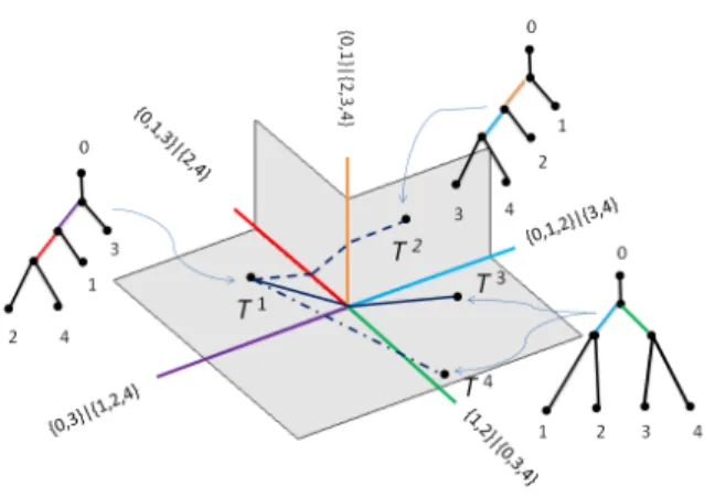
1.1 (a) shows the brain blood vessel system of a person. (b) illustrates one of the brain artery trees used as data objects in the present research. . . 1 1.2 A portion of T4 with three trees T1, T2, T3 and their projections onto the common edge.
Orange represents common edge, while blue, red, yellow represent non-common edges. Black lines illustrate the contractions of non-common edges. . . 4 1.3 Three examples of shortest paths in T4. All three paths are shortest paths between pairs of
trees. In particular, the solid line represents a cone path. . . 4 1.4 Comparison triangle . . . 5 2.5 (a) One slice of a Magnetic Resonance Angiography (MRA) image for one person. Bright
regions indicate blood flow. These are tracked through MRA slices to recover artery tubes as shown in the figure on the right. (b) The data object is a reconstructed brain artery tree for one person. The goal of this research is PCA type statistical analysis of a sample of such data objects. . . 17 2.6 Illustrates steps forcortical correspondence. (a) Brain artery system (blue) with the cortical
landmarks (red). (b) Find the closest point on the brain artery system to each landmark (red segments are landmark connections). Arteries which are not between the landmark projections and the base (cyan) are trimmed. (c) The result of this procedure is a cortical correspondence tree. . . 18 2.7 Schematic plots showing the three possibilities to insert a new leaf in the first iteration. . . . 20 2.8 Comparison between KDE of edge lengths in brain artery data (blue solid curve) and Gamma
distribution with parameters 1.28 and 15.8 (red dashed curve) shows the Gamma distribution is an excellent fit for the edge lengths distribution of the brain artery data. . . 20 2.9 (a) A template phylogenetic tree with 4 leaves and edge lengths in boxes. (b) The
correspond-ing population genealogical tree has the same topological structure as the template tree. The number of reproduction cycles in each subpopulation equals the corresponding edge length in the template tree and the size of subpopulation in each generation is the width parameter which equals 4. . . 22 2.10 Two possible sample gene trees generated within the same population genealogical tree, from
Figure 2.9(b). . . 23 2.11 Two possible sample gene trees with different topologies can be generated within the same
population genealogical tree, from Figure 2.9(b). . . 23 2.12 (a) Overlay of pairwise angle KDE plots shows the decreasing similarity ordering of the five
data sets: WF2, WF10, WF40, brain artery data, and uniformly random data. (b) Overlay of logarithm of pairwise angle KDE plots indicates that the variability in pairwise angles is proportional to the magnitude of angles for WF2, WF10, WF40, and brain artery data, but not for the uniformly random data. . . 25 2.13 (a) Overlay of pairwise distance KDE plots shows the decreasing similarity ordering of the five
3.14 The above scatter plot matrix gives a visualization of 3-D MDS configuration on 3 clusters from front, side, and top views. Both distance MDS and classical MDS produce this same
3-D configuration. Three data clusters are colored red, green, and blue. . . 31
3.15 Comparison across classical MDS, distance MDS, and PCA on 3-cluster (colored red, green, and blue) simulated data set. Shows low rank approximations of Euclidean data are different between classical MDS and distance MDS. . . 32
3.16 2-D MDS plots associated with 3 biological variables: age, gender and handedness. No clear correlates of these biological variables can be drawn. . . 33
3.17 3-D MDS plots in rainbow color scheme across ages along with top, side, and front views in separate sub-figures. Very limited information gained from adding the third dimension. . . . 33
3.18 3-D MDS plots with males in blue dots and females in green dots along with top, side, and front views in separate sub-figures. Very limited information gained from adding the third dimension. . . 34
3.19 Examples of embedding geodesics in 2-D MDS plots . . . 36
3.20 2-D MDS plots with one triangle embedded . . . 37
3.21 Examples of embedding geodesics as out-of-sample objects in 2-D MDS plots . . . 41
3.22 HDOS embedding of median length geodesic with embedding dimension p= 3,5,10,66 . . . . 43
3.23 HDOS embedding of median length geodesic with embedding dimension p= 3,5,10,66 . . . . 44
3.24 HDOS embedding of median length geodesic with embedding dimension p= 3,5,10,66 . . . . 46
4.25 The solid path denotesP(T1, T2) andP(T1, T2)6= Γ(T1, T2). The dashed ellipse represents the vistal cellV containingT∗, e T andT0. The dotted path betweenT1 andT0 together with the solid segment betweenT0 and e T is Γ(T1, e T). We reach a contradiction that there are two distinct geodesics betweenT1 andT∗. . . . 49
4.26 Examples of lines inT4 . . . 50
4.27 The above figure shows three geodesics in a portion of T4: Γ(T1, T2) is uniquely extendable and can be extended into a type I line; Γ(T1, T6) is also uniquely extendable but can not be extended into a type I line; Γ(T2, T6) is not even uniquely extendable. . . . 51
4.28 The above figure shows extensions of Γ(T1, T2) and Γ(T2, T3) which are uniquely extendable geodesics for the three trees in Figure 4.27. . . 52
4.29 The above figure gives a detailed view of what happens when Γ(T1, T2) crosses Oi−1∩ Oi which is intuitively represented by the central vertical axis in bold. . . 56
4.30 The above figure gives a detailed view of what happens wheneis contracted. . . 57
5.31 The above figures show the distributions of data projections along SLG1 across five data sets. The projections are only distributed within a relatively narrow range between the two end points of SLG1 for all five data sets. . . 65
6.33 The black dotted lines represent locally optimal rays, and the red circle denotes the Fr´echet mean. This plot shows that the locally optimal rays and the Fr´echet mean do not locate in the same orthant. . . 71 6.34 This figure shows the non-concavity of the objective function (6.12) as well as some other
aspects of this toy example inT4. The horizontal axis gives the angle travelled by the moving ray. The vertical axis represents the sum of squared projections from 10 data points onto the moving ray. The orthant boundaries are indicated by dashed vertical lines. The Fr´echet mean is plotted as the green vertical line. The blue curve shows how the value of the objective function changes as the ray moves. The red horizontal line segments keep track of which data points project positively onto the ray. . . 72 6.35 Red dots represent the sorted proportions of the total variation in the brain artery data
captured by 67 locally optimal rays which are returned by the steepest descent algorithm. Blue circles represent the sorted proportions obtained in the way that the squared norm of each tree is divided by the total squared norm of the brain artery data. The two plots are the same, which indicates that locally optimal rays go through trees in the data set. . . 75 6.36 Peterson graph illustrating how the steepest descent search algorithm works for the
landmark-reduced brain artery data set with only 5 leaves. All 85 data trees are contained in 5 orthants represented by dashed line segments. The search algorithm will end at locally optimal rays in different orthants depending on where the search process starts. . . 76 6.37 Bar graph showing the comparison of proportions of total variation captured by the best
locally optimal ray across 8 landmark-reduced brain data sets. . . 77 6.38 This plot shows that there will be a contradiction if tree T projects positively onto two
antipodal rays~r1 and~r2. . . 78 6.39 Shows the comparison of the four greedy approaches for three data sets: (a)Brain Artery data,
LIST OF TABLES
3.1 Row 1 gives the values for the embedding dimension p, and Row 2 shows the Stress of the 2-dimensional out-of-sample representation for each p. The Stress gets slightly larger as p increases, which indicates that the Stress of 2-dimensional representation is not a good measure of HDOS distortion. . . 44 3.2 Row 1 gives the values for the embedding dimension p, and Row 2 shows the Stress of the
p-dimensional out-of-sample representation. The Stress decreases as p increases, which is compatible with what we saw in Figure 3.22. . . 44 5.3 Column 1 shows the performance of SLG1 for five data sets without counting end points.
Column 2 shows the same statistics but counting end points. Column 3 lists the total variation with respect to the Fr´echet mean in each data set. Overall, SLG1 explains a relatively small amount of the total variation in all five data sets. . . 63 5.4 Column 1, 2, and 3 show the total variation with respect to the origin, the total variation
with respect to the Fr´echet mean, and the effect of the Fr´echet mean in each data set. . . 64 6.5 This table lists four summaries across five data sets and the proportion in the third column
is used to measure the performance of the best locally optimal ray. . . 73 6.6 Comparison of the proportions of data variation captured by the 1st PA set using 4 greedy
approaches across 5 data sets. Suggests that the forward approaches are better than the backward approaches in terms of capturing data variation. . . 82 6.7 Comparison of the numbers of antipodal axes in the 1st PA set using 4 greedy approaches
across 5 data sets explains what we have seen in Table 6.6. . . 82 6.8 Comparison of the numbers of PA sets needed to capture at least 80% of the data variation
CHAPTER 1: INTRODUCTION 1.1 Motivation
This dissertation focuses on Object Oriented Data Analysis in the context of tree-structured objects. The concept of “Object Oriented Data Analysis”(OODA) was first defined by [Wang and Marron, 2007] and has more recently been discussed in [Marron and Alonso, 2014]. Essentially OODA is the statistical analysis of a population of complex objects. In traditional statistical analysis, the atoms are generally either numbers or vectors. In functional data analysis, a currently active research area, each sample element is considered to be a function; see [Ramsay and Silverman, 2002, 2005] for a detailed review. Wang and Marron extended the idea of functional data analysis to even more complicated objects such as images, two-dimensional or three-dimensional shapes, and combinatorial structures such as graphs or trees.
In [Wang and Marron, 2007], the authors modeled the human brain blood vessel systems as binary trees. Two types of information were taken into account: topological structures and attributes associated with nodes. Although both that work and the present research are based on a common set of human brain blood vessel systems, very different aspects of the data are studied here. Figure 1.1(a) gives an example of such a blood vessel system. Each blood vessel system studied in the present research is oriented with respect to 128
(a) (b)
carefully chosen (i.e. to correspond across patients) landmarks on the cortical surface. As in [Skwerer et al., 2014a], the cortical correspondence method of [Oguz et al., 2008] gave the landmarks. All 128 landmarks are used as non-root nodes and an artificial conceptual point is defined to be the root node. Corresponding to each landmark, a closest point on the brain artery is found by minimizing the 3-D Euclidean distance from the landmark. Due to the natural tree-like structure of the brain artery system, a brain artery tree is formed by connecting each landmark with this closest point, and one example is given in Figure 1.1(b). For the tree representation in the present research, the edge lengths are considered as important geometrical information. This is different from [Wang and Marron, 2007] in which the authors used nodal attributes containing other geometrical summaries.
Many applications of OODA come from the field of medical image analysis. In [Singh et al., 2010], researchers took brain shapes as objects and applied Partial Least Squares Regression to characterize the neuroanatomical variations observed in neurological disorders. In [Geneser et al., 2011], lung shapes were taken to be the objects and researchers modeled the changes in lung shapes as a function of chest wall amplitudes to calculate the resulting variability in radiation dose accumulation.
The present research is performed under the framework of phylogenetic tree space which was first built in [Billera et al., 2001]. In this space, there is a unique shortest path between each pair of trees, called a geodesic. Later [Owen and Provan, 2009] constructed a polynomial time algorithm to compute the geodesic distance which is implemented in [Skwerer, 2014]. These works enable us to find projection of one tree onto a subset of trees in phylogenetic tree space, and furthermore makesPrincipal Component Analysis (PCA) possible in this space.
1.2 Phylogenetic Tree Space
The foundation of this research was developed by [Billera et al., 2001], which gave a rigorous geometric definition of the space of rooted labeled trees. We will start this section with introducing some of the basic concepts in graph theory.
1.2.1 Phylogenetic n-trees
We are using standard graph theory terminology, such as given in [Ahuja et al., 1993; Bazaraa et al., 2010; Cormen et al., 2009]. A tree T is a connected graph with no cycles. A node of T is called a leaf if there is a unique edge connected to it, and the edge is called aleaf edge. V ={0,1, . . . , n} usually denotes the leaf set of T. A weighted tree is a tree with each edge e assigned a weight |e|, or |e|T if we want to
emphasize the treeT to whichebelongs. An edgeeiscontracted if|e|= 0. Asplit associated with edgeeis defined asσe=Ve|Ve, whereVe,Veare sets of leaves andVe|Verepresents the partition ofV resulting from
property that one of the setsVeTVf,VeTVf,VeTVf, orVeTVf is empty. This concept can be naturally
extended to the compatibility of two sets of edgesAandB: if for each edgee∈A and each edgef ∈B,e is compatible withf, then we sayAandB are compatible. Here is some facts about compatibility:
• Each edge is identified uniquely by its split, henceforth edges from different trees with the same set of leaves are comparable.
• Each pair of edges in a tree are compatible.
• A tree is determined uniquely by its set of splits.
A phylogenetic n-tree (or simply n-tree) is a weighted tree T = (V,E, W,Σ), where V = {0,1, . . . , n} is a labeled set of leaves (with 0 arbitrarily denoting the root of T), E is the set of interior (non-leaf) edges, W ={|e|:e∈ E}is the set of edge weights which is also the set of edge lengths, and Σ ={σe:e∈ E}is the
set of splits forT.
In an n-tree, all the non-leaf nodes are assumed to have at least 3 adjacent edges. Amaximal n-tree is an n-tree with the largest number (2n−1) of edges, or the largest number (n−2) of interior edges. Since all trees with the same set of leaves contain the same set of leaf edges, we will ignore them in this dissertation that follows. Notice that every n-tree can be represented topologically by contracting a set of edges from some maximal n-tree.
1.2.2 Construction of Phylogenetic Tree Space
Phylogenetic tree space, ortree spaceTn is a geometric space in which each point represents an n-tree and
is placed in an (n−2)-dimensionalorthant(copy ofRn−+ 2) with each orthant associated with some maximal n-tree. Orthants are attached to each other through common edges. Here we denote an orthant associated with treeT = (V,E, W,Σ) asO(E). Tree space is thus a union of (2n−3)!! orthants [Schr¨oder, 1870], each of which corresponds to a distinct maximal tree topology. For any two treesT1andT2inT
n,d(T1, T2), the
distance betweenT1 andT2, will be defined as the length of the shortest path connecting them inT
n. This
extends the standard Euclidean metric, which is the standard distance between two vectors.
a projectionPionto the vertical line by contracting its non-common edge as shown by black lines in Figure 1.2.
Figure 1.2: A portion ofT4with three treesT1,T2,T3and their projections onto the common edge. Orange represents common edge, while blue, red, yellow represent non-common edges. Black lines illustrate the contractions of non-common edges.
Figure 1.3: Three examples of shortest paths inT4. All three paths are shortest paths between pairs of trees. In particular, the solid line represents a cone path.
Tree space has properties that are very useful for deriving and constructing statistical properties in the space. One important property noted in [Billera et al., 2001] is that Tn is a non-positively curved,
or CAT(0) space. Intuitively speaking, every triangle in a CAT(0) space is skinnier than a triangle with exactly the same lengths of sides in Euclidean space. More precisely, a metric spaceX is said to beCAT(0) if the following statement is true. Given any three points a, b and c, as illustrated in Figure 1.4, with distances d1 =d(b, c),d2 =d(a, c), and d3 =d(a, b), form a “comparison triangle” in the Euclidean plane. The “comparison triangle” has vertices a0, b0, and c0 with side lengths d1 = d(b0, c0), d2 = d(a0, c0), and d3=d(a0, b0). Ifxis a point on the geodesic fromatob, at distanced4froma, find the corresponding point x0 on the straight line froma0 to b0 at distanced4 from a0. Then d(x, c)6 d(x0, c0). This leads to many useful consequences as seen in the next section.
Figure 1.4: Comparison triangle
1.3 Construction of Geodesics
Because the tree space is CAT(0), it follows by [Gromov, 1987] that there is a unique shortest path connection any two points T = (V,E, W,Σ) and T0 = (V,E0, W0,Σ0) of T
n, called the geodesic Γ(T, T0)
betweenT andT0, and its length d(T, T0) can be used to define a metric in tree space. This is the metric defined by [Billera et al., 2001]. This section reviews the topological structure of Γ(T, T0) and the algorithm given by [Owen and Provan, 2009] to compute d(T, T0). The topological structure of a geodesic was first given in [Billera et al., 2001] which showed that Γ(T, T0) is a piecewise linear path contained in a sequence of orthants. Each linear portion of Γ(T, T0) is called aleg, and the sequence of orthants is called apath space
P associated with Γ(T, T0). Assume there arek+ 1 orthantsO0,O1, . . . ,Ok in P, and letC denote the set
of common edges betweenT andT0. Now let A= (A1, . . . , Ak) andB= (B1, . . . , Bk) be partitions ofE \ C
andE0\ C, respectively, such thatA
i andBjare compatible for eachi > j. Then (A,B) is called thesupport
ofP, andA1∪A2∪ · · · ∪Ak∪ C is the edge set associated withO0 andB1∪ · · · ∪Bi∪Ai+1∪ · · · ∪Ak∪ C
is the edges set ofOi for 16i6k. Some properties about path space have been clarified further in [Owen,
Since the Euclidean metric is preserved within each orthant ofTn, the geodesic Γ(T, T0) will consist of a
series of straight line segments through the orthants of the path spaceP. The properties of Γ(T, T0) will be
given in Theorem 1.3.1 which is the combination of Theorem 2.2, Theorem 2.3, Theorem 2.4 and Theorem 2.5 in [Owen and Provan, 2009]. For a setAof edges, we use||A||=pP
e∈A|e|2 to denote the norm of the
vector whose components are the lengths of the edges inA.
Theorem 1.3.1. Let T = (V,E, W,Σ) and T0 = (V,E0, W0,Σ0) be two n-trees. Let C be the set of edges
which are common to both trees, and let P be a path space containingT and T0 with support(A,B) of all the non-common edges. Then (A,B) corresponds to a geodesic if and only if it satisfies the following three properties:
(P1) For eachi > j,Ai andBj are compatible.
(P2) kA1k
kB1k ≤
kA2k
kB2k ≤. . .≤
kAkk
kBkk.
(P3) For each support pair(Ai, Bi), there is no nontrivial partitionC1∪C2 ofAi, and partition
D1∪D2 ofBi, such thatC2 is compatible withD1 and kCkD11kk < kCkD22kk.
Further let Γdenote the geodesic between T andT0, and parameterizeΓasΓ = (γ(λ) : 0≤λ≤1)where λis the ratio of distance to T. In this way,Γ can be represented inTn with legs
Γi=
h
γ(λ) : λ
1−λ ≤ kA1k
kB1k
i
, i= 0
h
γ(λ) : kAik
kBik ≤
λ
1−λ ≤ kAi+1k
kBi+1k
i
, i= 1, . . . , k−1,
h
γ(λ) : λ
1−λ ≥ kAkk
kBkk
i
, i=k
where the points on each legΓi are associated with the treeT
i= (V,Ei, Wi,Σi)having edge set
Ei = B
1∪. . .∪Bi∪Ai+1∪. . .∪Ak∪ C
and where the edge lengths in Wi are given by
|e|Ti =
(1−λ)kAjk−λkBjk
kAjk |e|T e∈Aj
λkBjk−(1−λ)kAjk
kBjk |e|T
0 e∈Bj
(1−λ)|e|T +λ|e|T0 e∈ C .
L(Γ) =
kA1k+kB1k, . . . ,kAkk+kBkk, s
X
e∈C
(|e|T − |e|T0)2
(1.1)
whereC is the set of common edges in the corresponding trees.
We note that geodesics can trivially be extended to include leaf edges, since these are always common to both trees and thus will be elements ofC.
In the above Theorem 1.3.1, the combination of (P1) and (P2) only gives us a necessary but not sufficient condition for a (T, T0)-path with support (A,B) to be a geodesic, and (P3) focuses on characterizing when this path is guaranteed to be a geodesic by specifying when no local improvement can be made for the path. Based on this theorem, anO(n4) algorithm was developed in [Owen and Provan, 2009] and a Java implementation of the algorithm is available at http://www.stat-or.unc.edu/webspace/miscellaneous/provan/treespace. 1.4 The Fr´echet Mean
One of the important applications of the geodesic algorithm is computing the Fr´echet mean. For most data sets, notions of center of data, such as the mean or median provide useful descriptive statistics. For data sets in tree space though, it is challenging to define analogous objects, since trees can neither be ordered nor operated on as Euclidean points. If we only take into account the structure information of trees but no edge length, then identifying a single “best” representative for a set of trees is well-studied in phylogeny, and such trees are usually called “consensus trees”. Consensus trees are difficult to calculate, however, and do not tend to take edge lengths into account effectively. TheFr´echet mean is a more promising candidate for measuring the center of a set of trees.
The Fr´echet mean is characterized as the solution to a non-linear optimization problem. For a set of pointsT={T1, T2, ..., Tr} inTn theFr´echet function F :Tn →R≥0 is the mean square distance
F(T) = 1 r
r X
l=1
d(T, Tl)2
whered(·,·) is the geodesic distance, and theFr´echet mean is
¯
T =argminT∈TnF(T).
The Fr´echet mean ¯T is unique because Tn is CAT(0) and d(T, T0) is a convex function of T for fixed T0
dataset.
Since the Fr´echet mean is such a useful summary statistic for tree data, it is worth some effort to review theinductive mean algorithmpresented by [Sturm, 2003, Theorem 4.7], and further analyzed in [Ba˘c`ak, 2012] and [Miller et al., 2015]. Given a set of treesT = {T1, T2, . . . , Tr}, let {Y
1},{Y2}, . . . denote a sequence of independently and identically distributed random trees chosen uniformly from T. Then the following sequence of trees converge to the Fr´echet mean of T:
S1:=Y1,
and
Sk:=
1−1 k
Sk−1+ 1 kYk,
where the right hand side of the second equation denotes the point 1
k of the distance along the geodesic
fromSk−1toYk. The pointSk is called thekthinductive mean ofY1, . . . , Yk. Theorem 4.7 of [Sturm, 2003]
states that this inductive mean converges to the Fr´echet mean for data sampled from any CAT(0) space. In particular, the expected squared distance between Sk and ¯T is bounded by F( ¯T)/k. This is also the
theoretical foundation of the following inductive mean algorithm in [Ba˘c`ak, 2012]. Inductive Mean Algorithm
Input:{T1, T2, . . . , Tr} Step 1 S1:=T1,i:= 1
Step 2 choose k∈ {1, . . . , r} at random Step 3 Si+1:=i+11 Tk+i+1i Si
Step 4 i:=i+ 1 Step 5 go to Step 2
1.5 The Combinatorics of Geodesics
Geodesics play an essential role in tree space data analysis and this section summarizes some useful results about the combinatorial structure of geodesics inTnfrom [Miller et al., 2015, Section 3]. Fix a source
tree T ∈ Tn, and consider the geodesic ΓX = Γ(T, X) from an arbitrary tree X ∈ Tn to T. ΓX has a
combinatorial structure specified by the support pair (A,B) associated with the geodesic. This support pair can change even whenX stays in the same orthant, depending on the precise values of the edge lengths in X. Miller et al. constructed a partition ofTn into regions for which all geodesics to the fixed treeT have the
same combinatorial structure. This partition is called the vistal subdivision ofTn and its major properties
Definition 1.5.1. [Miller et al., 2015, Definition 3.1] Given a source treeT ∈ Tn, a maximal orthantO ⊂ Tn,
and a support (A,B), letV(T,O;A,B) be the closure of the set of trees{X∈ O}for which the geodesic ΓX
joining each X to T has support (A,B) satisfying (P2) and (P3) with strict inequalities. Aprevistal facet is any nonempty setV(T,O;A,B) of this form.
The description of V(T,O;A,B) becomes linear after a simple change of variables. For convenience in notations, the treeX = (V,E, W,Σ) can be thought of as a vector in RE+, whose coordinates are expressed using the corresponding lower-case letterx.
Definition 1.5.2. [Miller et al., 2015, Definition. 3.2] Thesquaring mapTn→ Tn acts onX ∈ Tn⊂RE+by squaring the coordinates ofX:
(xe|e∈ E)→(ξe|e∈ E), whereξe=x2e
Denote byT2
n the image of this map, and letξe=x2edenote the coordinate indexed bye∈ E. The image
of an orthant inTn is then the equivalent orthant in Tn2, and the image of a previstal facet V(T,O;A,B)
in T2
n is avistal facet denoted byV2(T,O;A,B). With this change of variables, given any edge set S⊂ E,
kSk=P e∈Sξe.
The squaring map induces on the Fr´echet functionF a corresponding pullback function
F2(ξ) =F(pξ), where(pξ)e= p
ξe.
Since the Fr´echet functionF(T) is continuous on Tn with a uniquely attained minimum by convexity, and
continuously differentiable on the interior of every maximal orthant, the same properties hold forF2. Thus descent methods apply after squaring just as beforehand.
Proposition 1.5.1. [Miller et al., 2015, Proposition 3.3] The vistal facetV2(T,O;A,B)is a convex polyhe-dral cone inT2
n defined by the following inequalities onξ∈Rn−2, where all norm k · kare to be interpreted
ask · kT.
(O) ξ∈ O; that is,ξe≥0 for alle∈ E, andξe= 0fore /∈ E, whereO=Rn−≥02.
(P2) kBi+1k2 X
e∈Ai
ξe≤ kBik2 X
e∈Ai+1
ξe for alli= 1, . . . , k−1.
(P3) kBi\Jk X
e∈Ai\I
ξe≥ kJk X
e∈I
ξe for all i = 1, . . . , k and subsets I ⊂ Ai, J ⊂ Bi such that I∪J is
Remark: (P2) and (P3) here are actually the same as (P2) and (P3) in Theorem 1.3.1, but written in the form of multiplication instead of fraction. (O) is just a nonnegativity constraint.
Proposition 1.5.2. [Miller et al., 2015, Proposition 3.4] The vistal facets are of dimension 2n−1, have pairwise disjoint interiors, and coverT2
n. A pointξ∈ Tn2 lies interior to a vistal facetV2(T,O;A,B)if and
only if the inequalities in (O), (P2), and (P3) are strict.
Definition 1.5.3. [Miller et al., 2015, Definition 3.5] Fix a source treeT ∈ Tn, a (not necessarily maximal)
orthant O ⊂ Tn, and a support (A,B). A signature associated with the support (A,B) is a length k−1
sequenceS= (s1, . . . , sk−1) of symbolssi∈ {=,≤}. Theprevistal cell defined byO,A,B, and S is the set
V(T,O;A,B;S) of points{X ∈ O}for which the ratio sequence for (A,B) at each pointX has the following specific form:
kA1k kB1ks1
kA2k
kB2ks2. . . sk−2
kAk−1k kBk−1k
sk−1 kAkk
kBkk
.
Thevistal cell V2(T,O;A,B;S)⊂ T2
n is the image ofV(T,O;A,B;S) under squaring.
Note that vistal cells are convex polyhedra. A canonical description of vistal cells is given in [Miller et al., 2015, Theorem 3.23].
Theorem 1.5.3. Fix a treeT ∈ Tn.
1. Vistal cells associated with geodesics toT are exactly those of the formV2(T,O;A,B;S), where (A,B) is a valid support sequence for(O, T)andS is a signature on(A,B). Here a signature is a list of ”=”, ”<”, and ”≤” symbols in (P2).
2. The dimension of a vistal cell V(T,O;A,B;S) isdim(O)−m(S), where m(S) is the number of ”=” components inS.
3. The representation by a valid support sequence and signature is unique up to reordering the support sets within each equality subsequence of S.
Definition 1.5.4. [Miller et al., 2015, Definition 3.31] Apremultivistal cell for a collectionTof trees is a set of the form
V(T;O;AT,BT) = r \
l=1
V(Tl,O;Al,Bl),
whereV(Tl,O;Al,Bl) are previstal cells, andO ⊂ T
n is an orthant, and
is a collection of support pairs for (Tl, T)-geodesics. A multivistal cell (m-vistal) is the image in T2
n of a
premultivistal cell.
1.6 PCA in Euclidean Space
Principal component analysis(PCA) has been a workhorse method for understanding population structure of a data set in Euclidean space. A good overview and discussion of many aspects of PCA can be found in [Jolliffe, 2005]. A common goal of PCA isdimension reduction: finding principal components out of the original set of variables and making sure the number of principal components is less than the number of original variables. There arepopulation principal components andsample principal components. Since we mainly deal with a sample of trees rather than the entire tree population in this research proposal, only the sample PCA (see [Mardia et al., 1979]) will be studied here. LetX = (x1, . . . , xn)0 be an n×psample
data matrix, i.e. the rows ofX are the data objects. Letabe a standardizedp-vector, i.e. a0a= 1. Since
variation is reasonably defined around a center point, we work with a mean centered version of the data, X−1¯x0, where1is ann×1 vector with all entries equal to 1 and ¯x0is a 1×pvector with theithentry being
the mean for the column iin X. Then the standard linear combination (SLC)Xa gives n observations on a new variable defined as a weighted sum of the columns of X. The sample variance of this new variable is a0Sa, whereS is the sample covariance matrix of X. The first result is that the SLC with largest variance is the first principal component defined by
y(1)= (X−1¯x0)g(1) (1.2)
where g(1) is the standardized eigenvector corresponding to the largest eigenvalue of S (i.e. S = GΛG0). Similarly, fori= 2,3, . . . ,theithsample principal component is defined as
y(i)= (X−1¯x0)g(i) (1.3)
whereg(i)is the standardized eigenvector corresponding to theithlargest eigenvalue ofS. And we have the following properties for principal components:
– The principal components are uncorrelated and the variance ofy(i) isλi, theith largest eigenvalue ofS.
– Among all the SLCs of columns ofX which are uncorrelated with the firstk principal components ofX, the (k+ 1)th principal component has largest variance.
– If S has rank r < p, then the total variation of X can be entirely explained by the first r principal components.
1.7 PCA on Manifolds
As noted in [Marron and Alonso, 2014], an interesting extension of PCA is to the “mildly non-Euclidean” setting, such as data objects on a manifold. The value of thinking about data on a curved manifold was first motivated in the area of directional data (i.e. the data objects are angles). Such data objects arise in many contexts, such as wind directions, magnetic directions, etc. Some good examples can be found in [Fisher, 1995; Fisher et al., 1993; Mardia, 1972]. To illustrate the motivation of thinking about directional data as lying on a manifold, we will take the following example from [Marron and Alonso, 2014]. Consider a data set consisting of four angles, 1◦, 2◦, 358◦, 359◦, and consider their average. By the fact that there are just four numbers, it is natural to compute the classical arithmetic mean. The result here of 180◦ is typically
not satisfactory if we view the angles as points on the unit circle. From this perspective a mean of 0◦makes more sense. The idea behind this toy example is: we think of paths between data points on a manifold as “moving along a surface using geodesics”.
As there are quite a few notions of data center in Euclidean space (such as mean, median, trimmed means, and so on), there are also many ways of defining center on manifolds. On a curved manifold, the Fr´echet Mean (see section 1.4) is one of the commonly used descriptions of data center. To measure the variation about center within a data set on a manifold, there are plenty of analogs of PCA. We will start with a simple one in the sense that it only requires a metric, calledMulti-Dimensional Scaling (MDS) [Borg and Groenen, 2005; Cox and Cox, 2001; Lingoes et al., 1979; Young and Hamer, 1987]. MDS takes a matrix of pairwise distances between data points and finds a lower dimensional representation of the data so as to optimize the relationships indicated by the distance matrix. The main advantage of MDS is that it works not only for manifold data but also for general metric space data. One major disadvantage of MDS is that it can be difficult to interpret. That is also why other generalizations of PCA for manifolds have been presented in the literature.
and get the PCA there, and then map the results back into the manifold. One concern about PGA is that the principal geodesics are constrained to go through the Fr´echet mean. It was shown in [Huckmann et al., 2010] that this was a serious constraint by using an example of uniformly distributed data points along the equator on the sphereS2. The Fr´echet mean of the data are the north and south poles, so PGA could only find a line of longitude which gives a poor representation of the data. To address this issue [Huckmann et al., 2010] proposedGeodesic Principal Components which finds the best fit over all geodesics.
On the sphereS2, by relaxing the constraint of searching within only geodesics, [Jung et al., 2011] pro-posed Principal Arc Analysis (PAA). PAA was motivated by the data following closely to a small circle (meaning not a great circle). In this case, the above modifications of PCA need to find at least two compo-nents to explain the variation. However, the nature of the data is still one dimensional, so having more than one component is unsatisfying. PAA addresses this by finding the best fit of any small circle to the data. Later on, [Jung et al., 2012] extended the idea of PAA to data lying on higher dimensional spheres, i.e. Sd,
whered >2, which is calledPrincipal Nested Spheres(PNS). The main idea behind PNS is iterative dimen-sion reduction. For addressing the problem that data objects lie in the Cartesian product of many spheres, [Pizer et al., 2012] proposed the method ofComposite Principal Nested Spheres (CPNS). The approach of CPNS is to do a sphere by sphere decomposition of the data using PNS, then to combine the scores into a large Euclidean vector, and finally to apply PCA to a collection of such large vectors.
1.8 PCA of Tree Structured Data Objects
[Marron and Alonso, 2014] pointed out that a more challenging extension of PCA is to “strongly non-Euclidean” settings, such as tree-structured or graph-structured data objects. Several attempts at extending PCA into tree structured data have already been made in literature. An early approach to the tree structured data PCA was in [Wang and Marron, 2007] where the statistical use of the term OODA first appeared. In that approach, the focus was on topological structure. Given a set of trees, a two-step procedure was performed: first, an optimal nested sequence of trees, calledprincipal structure treeline, was obtained; second, for each tree in the principal structure treeline, an optimalprincipal attribute treelinewas calculated (attributes being only on nodes). This line of research was continued in [Aydin et al., 2009a]. Aydin et al. used the term of principal structure treeline from [Wang and Marron, 2007] as their foundation, and one of their main contributions is a linear time computational method for a production scale data set of trees.
the topic of the first principal component in tree space. The basic idea of defining the first PC is closely related to the idea of [Wang and Marron, 2007]:
1 Given a set of trees{T1, T2, . . . , Tr}, construct a centerT0.
2 Given a geodesicπthroughT0, project{T1, T2, . . . , Tr}ontoπby finding the closest point y
i inπtoTi
fori= 1, . . . , n.
3 Find the geodesicπsuch that the pointsyi have the greatest variance along the geodesic.
In step(1), Nye chooses the centerT0to be themajority consensus tree[BARTH ´EL ´EMY, 1986]. The majority consensus topology consists of splits which are found in strictly more than half the trees in the data set. Due to the highly complex combinatorial features of tree space, it will be very computationally intense to directly follow the above procedure since it is not possible to try all the geodesics passing through the center. A natural idea is to come up with some good heuristics with acceptable computational complexity. The major contribution of [Nye, 2011] is to propose a greedy algorithm “ΦPCA” which computes an approximated first principal component. For the detail of the algorithm, see [Nye, 2011, Section 2]. The main idea of ΦPCA is that the principal component is constructed greedily by adding one coordinate in each step instead of all at once. Intuitively speaking, Nye reduces the problem of finding the direction with largest projection variance in an n-dimensional space into a series of 2-dimensional subproblems. This fundamental work of Nye is pioneering in tree space, but this area needs more comprehensive investigation due to interesting and complex topological structure.
1.9 Overview of Dissertation
CHAPTER 2: REAL AND SIMULATED DATA
There are several data sets which will be used through out the rest of this thesis to test and contrast the methods being developed. The purpose of this chapter is to highlight relevant aspects of several test bed data sets in order to enhance intuitive understanding of the numerical studies. In Section 2.1 the source of the brain artery data and the generation of the corresponding tree data set is discussed. Section 2.2 describes the generation of random tree data sets. In Section 2.3 the Wright-Fisher model, which is a useful tool to generate topologically similar trees, is considered. Useful contrasts between these example data sets are given in Section 2.4, using some exploratory data analyses. At the end of this chapter, a method of generating reduced brain artery data sets will be proposed.
2.1 Brain Artery Data
One of the original motivations in this thesis is to look for latent correlates of biological variables such as sex, age, and handedness from a set of human brain artery trees. Those brain artery trees were constructed from a raw data set of Magnetic Resonance Angiography (MRA) brain images collected by the CASILab at the University of North Carolina at Chapel Hill. The data set is publicly available and can be downloaded following the link on the MIDAG website [Bullitt et al., 2008]. See [Bullitt et al., 2005] for a simple summary based analysis of this image database. The full data set contains images of the brains of 109 healthy subjects and each image is tagged with subject features of age, sex, handedness and self-identified race.
2.1.1 Magnetic Resonance Angiography
(a) (b)
Figure 2.5: (a) One slice of a Magnetic Resonance Angiography (MRA) image for one person. Bright regions indicate blood flow. These are tracked through MRA slices to recover artery tubes as shown in the figure on the right. (b) The data object is a reconstructed brain artery tree for one person. The goal of this research is PCA type statistical analysis of a sample of such data objects.
one reconstructed 3-D artery system. An important point is that MRA has a resolution threshold of about 1mm. Consequently many small arteries, between 1mm in diameter down to capillaries, are too small for detection.
A challenge in this study is the starting point of the artery tree. For uniformity we work with a set of subtrees, where each subtree starts at the Circle of Willis, see [Aydin et al., 2009b]. The major part of this research develops PCA type statistical methods for the tree data set by using the phylogenetic tree space as a mathematical foundation. Recall from Section 1.2.2, a set of phylogenetic trees must have a common leaf set. However, the arteries detected by MRA do not even have the same number of branches across all the subjects. To address this issue, a common leaf set is artificially introduced by determining points on the cortical surface that correspond across different subjects. The next section describes the details of representing brain artery systems as points in phylogenetic tree space.
2.1.2 Cortical Correspondence
which are the red dots in Figure 2.6(a). For each landmark, the closest point on the artery tree system, called the landmark projection, is found. Each landmark is then connected to its landmark projection by a red segment in Figure 2.6(b). Each landmark and the line segment to its projection become part of the data object. Each phylogenetic tree data object is finally formed by tracing the parts of the tree that are between the base and the landmarks. Any parts of the original brain artery system that are not between a landmark projection and the base, found as cyan in Figure 2.6(b), are trimmed. The resulting tree is in Figure 2.6(c).
(a) (b) (c)
Figure 2.6: Illustrates steps for cortical correspondence. (a) Brain artery system (blue) with the cortical landmarks (red). (b) Find the closest point on the brain artery system to each landmark (red segments are landmark connections). Arteries which are not between the landmark projections and the base (cyan) are trimmed. (c) The result of this procedure is a cortical correspondence tree.
To form one tree instead of a few subtrees, an artificial leaf, called the root, is added to the base of the reconstructed data object to substitute for the Circle of Willis. The root and the 128 landmarks together add up to a common set of 129 leaves. Recall from Section 1.2.2, each edge of a reconstructed phylogenetic tree is associated with a positive edge length. The edge length for each interior edge is the corresponding arc length in the original brain artery system. The pendant for each landmark has length equal to the projection distance plus the original artery length from the projection point to the nearest artery branch. The pendant length for the root of the tree is zero.
Recall that the raw data set contains images of the brains of 109 healthy subjects. However, after performing cortical correspondence only 67 images produced eligible phylogenetic trees, hence the real data set will contain 67 brain artery trees throughout this thesis.
2.2 Generated Data Set I: Uniformly Random
phylogenetic trees with 129 leaves will be generated. Recall from Section 1.2.2 the fact that the number of all possible topologies for a tree with 129 leaves is 253!!≈10250.
(a) (b)
(c) (d)
Figure 2.7: Schematic plots showing the three possibilities to insert a new leaf in the first iteration.
the edge lengths of uniformly random trees will be generated from this Gamma distribution.
2.3 Generated Data Set II: The Wright-Fisher Model
Besides the random tree data set, some simulated data sets with controlled similarity of topology are also considered. Using the relationship between phylogenetic trees and genealogy, the Wright-Fisher model, introduced by [Wright, 1931] and [Fisher, 1930], will also be used to generate some test bed data sets in this thesis.
2.3.1 The Wright-Fisher Model
The basic concepts of the Wright-Fisher model are summarized in [Hein et al., 2005, Section 1.4]. The Wright-Fisher model is a simplified mathematical model of populations describing genealogical relationships. This model of reproduction provides a dynamic description of the evolution of an idealised population and the transmission of genes from one generation to the next. The following assumptions are made in the Wright-Fisher model:
1. Generations are discrete and non-overlapping.
2. The population is made of haploid organisms, that is, the genes making up the present generation are drawn randomly with replacement from the parental generation.
3. The population size is constant.
4. All individuals have equal reproductive ability.
5. The population has no geographical or social structure. 6. The genes (or sequences) in the population do not recombine.
genetic tree have the same population size and this single parameter is easy to control. From now on this parameter will be called thewidth parameter.
2.3.2 Data Generation
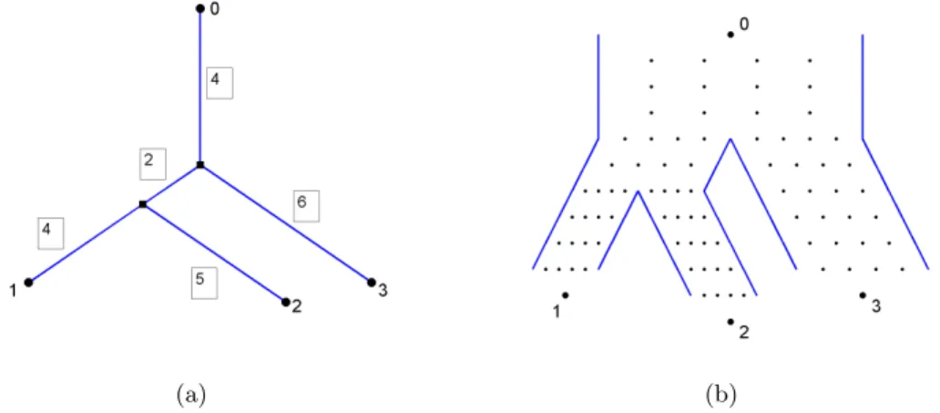
The actual data generating process starts from a template standard phylogenetic tree, with edge lengths assumed to be integer. (This may require the original lengths to be scaled or approximated.) This template tree is turned into a population genealogical tree which has the same topology, but additional attributes. A population genealogical tree preserves the edge lengths from the template tree by setting the number of reproduction cycles on each subpopulation to be the corresponding edge length in the template tree. To add population size as an additional uniform attribute on all edges, a population genealogical tree is constructed by choosing the population size equal to the predetermined width parameter. Figure 2.9(a) shows a template tree with 4 leaves and edge lengths as marked in boxes. Figure 2.9(b) gives the corresponding population genealogical tree with width parameter equal to 4. The population genealogical tree has the same topological structure as the template tree. Each horizontal line of dots represent a generation and the number of dots in each line equals the width parameter. The numbers of empty spaces between generations in each subpopulation reflect the edge lengths in the template tree. Each non-root leaf of the template tree becomes an individual from the latest generation of the corresponding subpopulation, and the root becomes the common ancestor of the whole population. Since the reproduction from generation to generation is random,
(a) (b)
Figure 2.9: (a) A template phylogenetic tree with 4 leaves and edge lengths in boxes. (b) The corresponding population genealogical tree has the same topological structure as the template tree. The number of repro-duction cycles in each subpopulation equals the corresponding edge length in the template tree and the size of subpopulation in each generation is the width parameter which equals 4.
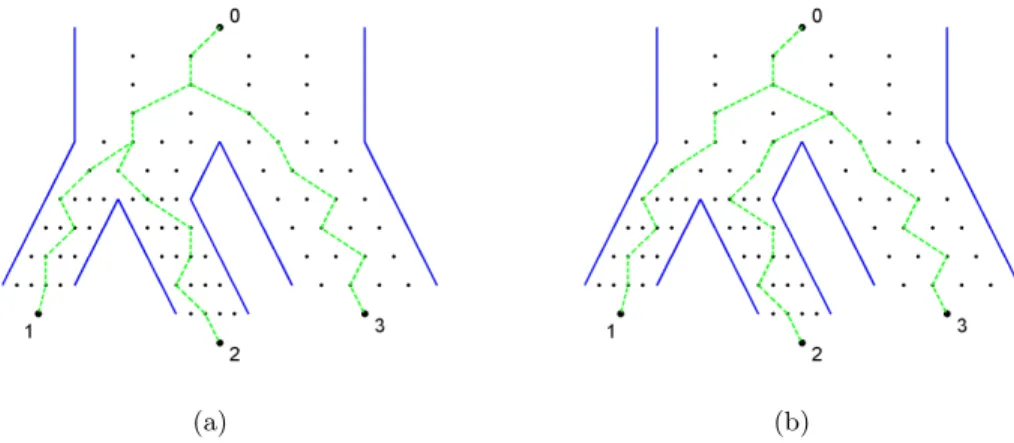
genealogical tree displayed in Figure 2.9(b). In both figures, three individuals labeled as 1, 2, and 3 have been randomly sampled in the most present generation of each subpopulation. Edges back in time tracking the ancestors of these three individuals are highlighted as green dashed lines. In (a) individuals 1 and 2 find a common ancestor first, then they find the common ancestor with 3. In (b) individuals 2 and 3 find a common ancestor first, then they find the common ancestor with 1.
(a) (b)
Figure 2.10: Two possible sample gene trees generated within the same population genealogical tree, from Figure 2.9(b).
To better visualize these two sample gene trees, we represent them in the form of phylogenetic trees in Figure 2.11 below. The phylogenetic tree in (a) corresponds to the sample gene tree in Figure 2.10(a), and it has the same topology as the template tree in 2.9(a). The phylogenetic tree in (b) corresponds to the sample gene tree in Figure 2.10(b), and it has a topology different from the template tree. Although the Wright-Fisher model can generate trees with topologies quite different from the template trees, they will tend to be “centered” around the original template tree. It is not known in what way the trees generated by the Wright-Fisher model statistically represent the original tree.
(a) (b)
2.4 Exploratory Data Analysis
In sections 2.1, 2.2, and 2.3, a variety of example data sets that will be used in later chapters are introduced. These are expected to exhibit different levels of similarity. We now focus on 5 specific cases, in order of decreasing similarity:
• WF2 (Wright-Fisher data with width parameter = 2) has a high level of similarity. • WF10 has similarity level lower than WF2 from Section 2.3.
• WF40 has even less similarity from Section 2.3.
• Brain artery data will be seen in Sections 2.4.1 and 2.4.2 to have less similarity than WF40.
• Uniformly random data will also be seen in Sections 2.4.1 and 2.4.2 to have the least similarity among all 5 cases.
2.4.1 Angle-based Data Summaries
One way to measure the similarity of tree data topologies is to study the distribution of angles, with vertex at the origin, between each pair of trees (calledpairwise angle). Given two treesT1 and T2, denote the pairwise angle between these two trees asθ, then we can defineθby the cosine law:
cosθ= kT
1k2+kT2k2−L(Γ(T1, T2))2
2kT1kkT2k . (2.4)
It can be shown that θ does not depend on either kT1k or kT2k. Under this definition, if Γ(T1, T2) is a cone path, thenθ= 180◦, otherwiseθ <180◦. A good general definition of angle in any metric space is the Alexandrov angle [Alexandrov, 1951]. In the special case of phylogenetic tree space, the definition of angle by the cosine law in (2.4) coincides with Alexandrov angle.
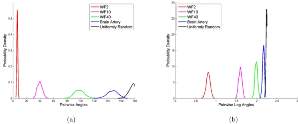
160◦ and a big proportion of angles are 180◦, showing the brain artery data set is not purely random. The overall comparison of these five distributions is consistent with the similarity ordering of these five data sets mentioned in the bullet points just before Section 2.4.1. Very often the spread of a data set is proportional to its mean, to investigate this issue, Figure 2.12(b) presents the overlay of the logarithms of the pairwise angles. Except for the uniformly random data, all other four data sets have similar spread, which indicates the variability in pairwise angles is proportional to the magnitude of angles.
(a) (b)
Figure 2.12: (a) Overlay of pairwise angle KDE plots shows the decreasing similarity ordering of the five data sets: WF2, WF10, WF40, brain artery data, and uniformly random data. (b) Overlay of logarithm of pairwise angle KDE plots indicates that the variability in pairwise angles is proportional to the magnitude of angles for WF2, WF10, WF40, and brain artery data, but not for the uniformly random data.
2.4.2 Distance-based Data Summaries
the distances between each tree and the origin differ for the brain artery data and the uniformly random data, probably because the distribution of edge lengths used in the uniform generation is different from the true distribution of the edge lengths in the brain artery data. This shows that it is worth looking at both pairwise angles and pairwise distances. Figure 2.13(b) presents the overlay of the logarithms of the pairwise distances, which again gives a good indication of proportionality between the spread and magnitude of pairwise distances.
(a) (b)
Figure 2.13: (a) Overlay of pairwise distance KDE plots shows the decreasing similarity ordering of the five data sets: WF2, WF10, WF40, brain artery data, and uniformly random data. (b) Overlay of the logarithm of pairwise distance KDE plots implies the proportionality between the spread and magnitude of pairwise distances.
2.5 Stickiness and Landmark-reduced Brain Artery Data
Fr´echet mean.
One goal of this dissertation research is to understand the effect of different aspects of a data set on the performance of our tree space principal components. Stickiness is certainly a potentially interesting aspect of tree space data. Since the suspected strong stickiness of the Brain Artery data and the Uniformly Random data is associated with their large data spread, ideally we want a series of data sets with different levels of spread. Fortunately, a group of landmark-reduced Brain Artery data sets with different levels of spread have been created and thoroughly studied in [Skwerer, 2014]. These data sets come from a slightly different data source from our Brain Artery data. Each of them contains 85 subjects instead of 67, but 64 of the 67 subjects in our Brain Artery data are included in those 85 subjects. In addition, the original set of 128 landmarks are chosen differently from our Brain Artery data. The landmarks of the 85-subject data are chosen by only considering the locations on the cortical surface, but the landmarks of the 67-subject data are chosen by taking into account both locations and curvatures. However, from the results in [Skwerer, 2014, Section 3.2], we clearly see different levels of data spread across these data sets, which is our focus here.
CHAPTER 3: MULTIDIMENSIONAL SCALING IN TREE SPACE
PCA type visualization is very helpful when dealing with high-dimensional complex data sets. A challenge of visualizing tree space is that it is strongly non-Euclidean. Multidimensional Scaling (MDS) gives one approach to addressing that. MDS is an analog of PCA, which is applicable in any metric space, such as tree space. It searches for a lower dimensional representation of a data set based only on pairwise distances defined between each pair of data objects. In Section 3.1, a brief review of MDS is given. In Section 3.2, 2-D and 3-D MDS are applied to the brain artery data set introduced in Chapter 2. In Section 3.3, it is seen that embedding one or more geodesics into a data set create a major distortion in the MDS, allowing study of how the geodesics behave in tree space. In Section 3.4, it is seen that an out-of-sample approach to MDS can mitigate this distortion.
3.1 Review of Multidimensional Scaling
In this section, we give a short introduction of MDS [Torgerson, 1952, 1958; Gower, 1966]. MDS finds an appropriate configuration in Euclidean space for a set of objects in any complex space as long as the dissimilarities between pairs of objects can be defined. Adissimilarity matrix, the most common input form of MDS, consists of dissimilarity data for each pair of objects. In the case of a metric space, the dissimilarity is taken to be distance, although MDS works in more general spaces. In this work, since we focus on tree space with a metric, the word “distance” will be used in most of this chapter. If the objects are labeled i = 1, . . . , N, the distances are given by Di,j and the distance matrix is given by D. MDS gives a good
understanding of the relationships between the N data objects, by visually representing them as a set of “configuration points”,x1, . . . ,xN ∈Rk, whose pairwise distanceskxi−xjkapproximate each corresponding
Di,j. The dimension k of the configuration space is arbitrary in theory, but k = 2,3,4 are usual for the
purpose of visualization.
of fit, called “distance MDS”. More recently, many variations of these ideas have been developed for a variety of applications, see [Borg and Groenen, 2005; Cox and Cox, 2001] for a good overview of this literature.
During decades of development, MDS has become a rich field in the literature. [Buja et al., 2008] suggests two dichotomies which give a clearer view of the whole topic. The first one is “metric MDS versusnonmetric MDS”: Metric MDS uses the actual values of the dissimilarities, while nonmetric MDS uses only their ranks [Shepard, 1962; Kruskal, 1964a]. Nonmetric MDS estimates an optimal configuration simultaneously with an optimal monotone transformation f(Di,j) of the dissimilarities. Because the effect of edge lengths is
taken into account in the tree space, the present research focuses on the metric MDS. The second dichotomy categorizes metric MDS into either classical metric MDS or distance metric MDS. Since we are going to focus mainly on metric MDS in this research, the terms “distance MDS” and “classical MDS” will be used instead of “distance metric MDS” and “classical metric MDS” in the rest of this chapter. The main difference between classical MDS and distance MDS is the loss function used in optimizing the MDS configuration. A loss function is a commonly used tool to measure the lack of fit between dissimilarities Di,j and fitted
distanceskxi−xjk. For metric MDS,Stress andStrainare two most frequently used loss functions.
Distance MDS uses Stress as the loss function which is a direct measure of disparities between dissimi-larities Di,j and corresponding fitted distanceskxi−xjk. In the simplest case, Stress is a residual sum of
squares:
StressD(x1, . . . ,xN) =
X
i6=j=1...N
(Di,j− kxi−xjk)2 1/2
(3.5)
Then distance MDS will minimize Stress over all possible configurations (x1, . . . ,xN)T. The minimization
can be carried out by applying standard gradient descent to StressD, which can be viewed as a function on
RN k.
Classical MDS uses Strain as the loss function and the idea of Strain originates from recovering a set of points in Euclidean space [Torgerson, 1952, 1958; Gower, 1966]. Some basic results about classical MDS are summarized here from [Borg and Groenen, 2005; Cox and Cox, 2001]. Given an N×N matrix of squared Euclidean distancesD2E, we want to find the MDS coordinate matrixX ofx1, . . . ,xN ∈Rk up to a rotation
or reflection. The matrixX hasN rows, corresponding to theN objects. The number of columns ofX can be taken to be anyk6n−1. Since distances do not depend on locations, we can assume thatX has column means equal to zero to prevent arbitrary translation. In Euclidean space, there is an identity relating the distancekxi−xjk and the inner producthxi,xji:
kxi−xjk2=hxi,xii −2hxi,xji+hxj,xji.
Let I denote the N ×N identity matrix, let e = (1, . . . ,1)T ∈
J =I− 1
Nee
T. From the above identity, the inner product matrix B
E =−12J D2EJ and this operation is
called double centering. Note that matrix multiplication by J on the left or right removes the mean from each column or row respectively. To find the coordinate matrixX, we factorBE by spectral decomposition,
BE =QΛQT = (QΛ1/2)(QΛ1/2)T =XXT. Classical MDS only differs from the above procedure by replacing
the matrix of squared Euclidean distances D2
E with the matrix of the more general squared dissimilarities
D2. We first obtain the inner product matrixB =−1 2J D
2J by double centeringD2. Then we compute the spectral decomposition of B = QΛQT, but this decomposition does not give us the coordinate matrix X
directly. Instead, the coordinate matrixX is given byX =Q+Λ1+/2, where Λ+is the diagonal matrix of the firstklargest eigenvaluesgreater than zero.
It needs to be pointed out that both distance MDS and classical MDS will get the same configuration up to a rotation or shift of origin if the given distances are Euclidean and the dimension of the MDS space is the Euclidean rank of the data. However, if the distances are not Euclidean, these two versions of MDS will behave very differently. Even when the dissimilarities are Euclidean, but the dimension of the MDS space is less than the Euclidean rank of the data, these two versions of MDS still perform differently in the following example shown in Figure 3.14. In 3-D Euclidean space, consider three multivariate normal distributions: N3((5,0,0)T,I),N3((0,5,0)T,I), andN3((0,0,5)T,I). From each of these three distributions, a sample of 10
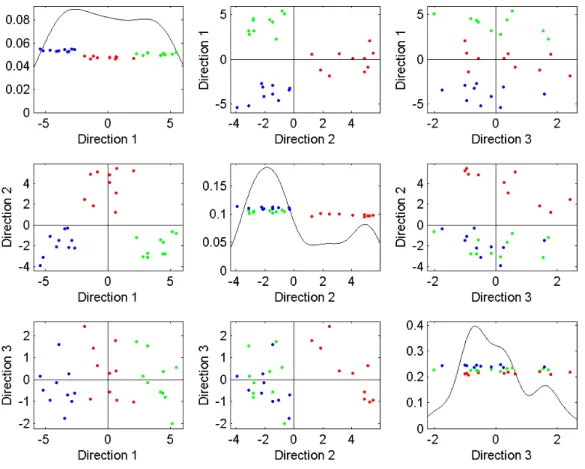
data points is randomly generated. Now we have three clusters of points in 3-D Euclidean space, colored red, green, and blue. Then an identical 3 dimensional MDS configuration is achieved by both distance MDS and classical MDS. For a better visualization, this common 3 dimensional MDS configuration is displayed in the form of ascatter plot matrix in Figure 3.14. The scatter plot matrix puts 1-D projections on the diagonals and corresponding pairwise projection scatter plots off the diagonals based on the three MDS directions. On the diagonals, there are three smoothed histograms of the data projections onto each MDS direction, of which the horizontal axes give the projection scores onto the three MDS directions and the vertical axes give the probability density of the projection scores. The first diagonal plot for MDS direction 1 shows a clear separation of three colors. The second diagonal plot for MDS direction 2 displays only a separation of red from green and blue, since it is orthogonal to direction 1. The third diagonal plot for MDS direction 3 shows no separation at all, because it is orthogonal to both directions 1 and 2. Consequently, the scatter plot of MDS directions 1 and 2 shows a perfect separation of the three original clusters. From the scatter plot of MDS directions 1 and 3, we can see that the three clusters are still kind of separated, but the separation is not as clear as for directions 1 and 2. Finally, the scatter plot of MDS directions 2 and 3 only separates red from green and blue.
Figure 3.14: The above scatter plot matrix gives a visualization of 3-D MDS configuration on 3 clusters from front, side, and top views. Both distance MDS and classical MDS produce this same 3-D configuration. Three data clusters are colored red, green, and blue.
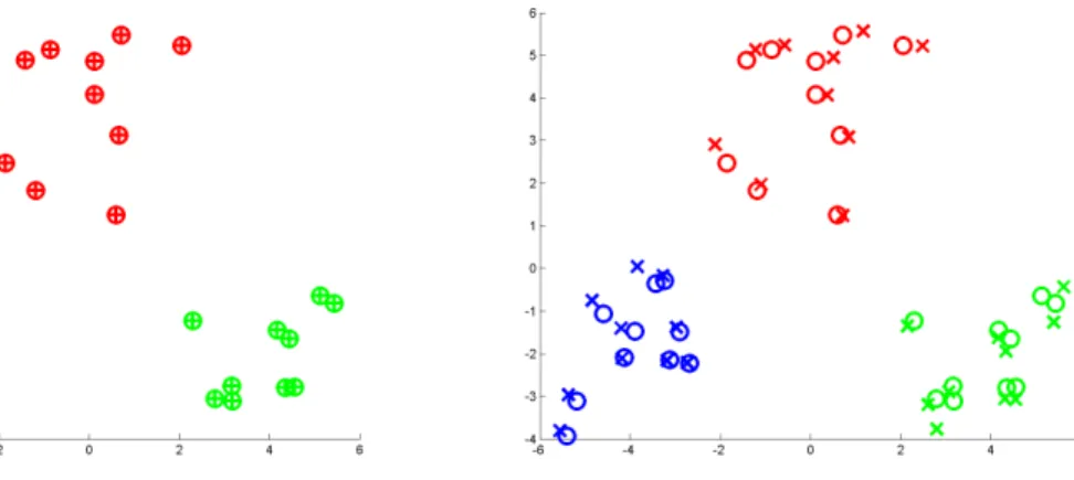
(a) 2-D classical MDS configuration is plotted us-ing “” and 2-D PCA configuration is plotted using “+”. The symbols of “” and “+” are perfectly overlapped, which indicates classical MDS and PCA are equivalent on Euclidean data.
(b) 2-D classical MDS configuration is plotted using “” and 2-D distance MDS configuration is plotted using “×”. The symbols of “” and “×” are not per-fectly overlapped, which indicates classical MDS and distance MDS perform differently even on Euclidean data.
Figure 3.15: Comparison across classical MDS, distance MDS, and PCA on 3-cluster (colored red, green, and blue) simulated data set. Shows low rank approximations of Euclidean data are different between classical MDS and distance MDS.
3.2 MDS of Tree Data
Recall one of the original motivations in this thesis is to search for potential correlates of biological variables such as sex, age, and handedness from a set of human brain artery trees. To better detect the potential classes, MDS is applied to aid visualization by embedding trees into a 2-D or 3-D Euclidean space. Recall MDS is based on the pairwise distance matrix of the data set. As in Section 1.3, distance between two trees is defined as the length of the geodesic connecting them, which can be computed by applying the linear time algorithm in [Owen and Provan, 2009]. Then MDS is performed on the geodesic distance matrix
e
conclusion can be made due to the small number of left-handed people. While it may be challenging to approximate a 126-dimensional data set by using a 2-dimensional configuration, the 2-D plot can still be a helpful visualization tool.
(a) 2-D MDS plot with ages in rain-bow colors: magenta for age 22, through blue, cyan, green, yellow, to red for age 72
(b) Same 2-D MDS plot with males in blue dots and females in green dots
(c) Same 2-D MDS plot with right-handedness in red dots and left-handedness in black dots
Figure 3.16: 2-D MDS plots associated with 3 biological variables: age, gender and handedness. No clear correlates of these biological variables can be drawn.
(a) 3-D MDS plot with ages in rainbow colors (b) MDS space dimension 1 vs dimension 2
(c) MDS space dimension 1 vs dimension 3 (d) MDS space dimension 2 vs dimension 3
The configuration space can be easily expanded into 3-D Euclidean space. The above Figure 3.17 shows a 3-D plot for the 67 brain artery trees in rainbow color scheme across age along with the orthographic views. Figure 3.17(a) shows a snapshot of the 3-D plot taken from a particular angle for the same data set in the above 2-D plot. Figure 3.17(b) shows the top view of Figure 3.17(a), which consists of the first and second dimensions in the MDS space and is also exactly the same plot as in Figure 3.16(a). Figure 3.17(c) and Figure 3.17(d) are the side view and front view of the 3-D plot in Figure 3.17(a). We are hoping to get better separation by introducing the third dimension in the MDS space, but the gain is quite limited.
The same visualization is shown for gender as well. Figure 3.18(a) shows a snapshot of the 3-D plot for the same data set. Figure 3.18(b), Figure 3.18(c), and Figure 3.18(d) show the top view, side view and front view of Figure 3.18(a) respectively. However, there is no apparent conclusion available about the separation between males and females.
(a) 3-D MDS plot with genders in different colors
(b) MDS space dimension 1 vs dimension 2
(c) MDS space dimension 1 vs dimension 3 (d) MDS space dimension 2 vs dimension 3
Figure 3.18: 3-D MDS plots with males in blue dots and females in green dots along with top, side, and front views in separate sub-figures. Very limited information gained from adding the third dimension.