01_ROBERTS_comparative-effects-mesh.pdf

(1)

Comparative effects of mesh resolution on

predictions of shallow water flow

Keith Roberts; Joannes Westerink

University of Notre Dame

(2)

Motivation

I How can we generate more efficient and objectively built multiscale meshes for shallow water flow solvers?

I The finite element mesh development process often is challenging and time consuming.

1. Accurate representation of boundaries while maintaining numerical stability.

2. Efficient and objective placement of resolution that does not exhaust your computing resources.

I Many model developers employ the expensive but reliable place-high-resolution-everywhere approach and run with a timestep between 0.25 s and 1 s.

(3)

Motivation: mesh-size function

We can target resolution with the use of a mesh-size function and an automated mesh generator.

I An isotropic mesh size function is a 2-D mapH(x,y) in which each (x,y) point has a corresponding mesh resolution or edgelength H.

I The mesh generator’s task is to construct a mesh that is faithful to H(x,y) quickly while ensuring a valid topology is produced.

wavelength slope feature size channels

H(x,y) mesh generator

Minimum of all

(4)

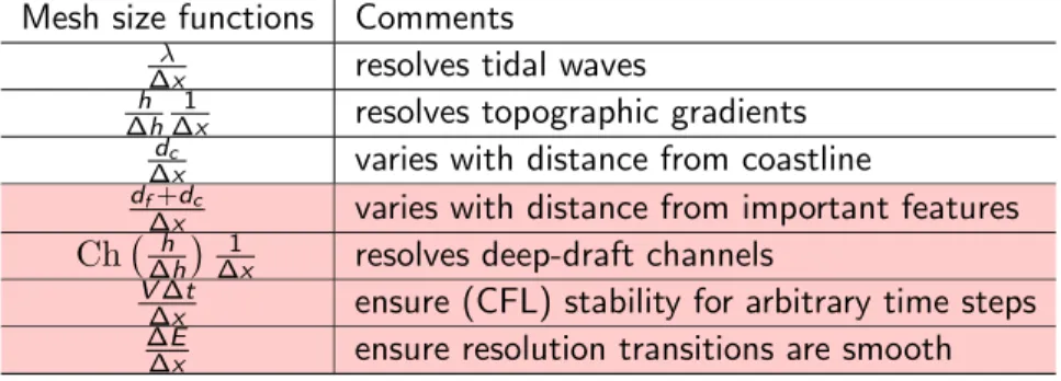
Mesh-size functions

I There are a handful of heuristics used to construct shallow-water flow models.

Table 1:Mesh size functions used to build reproducible and stable meshes. The red highlight indicates some more unique contributions.

Mesh size functions Comments λ

∆x resolves tidal waves h

∆h

1

∆x resolves topographic gradients dc

∆x varies with distance from coastline df+dc

∆x varies with distance from important features

Ch _∆h_h_∆1_x resolves deep-draft channels V∆t

∆x ensure (CFL) stability for arbitrary time steps

∆E

∆x ensure resolution transitions are smooth

(5)

Mesh generator: OceanMesh2D Library

I We 1_{have developed an open-source library (GNU license) in}

MATLAB (OceanMesh2D) to build 2D triangular meshes.

I Rapid (0.1-4 hours) build, validate, and modify workflows.

I This is the software that was used to build all the meshes in this work.

I It also contains post-processing scripts and accelerates common workflows (will be discussed on Friday).

Digital elevation model → 10 minutes stable mesh

1

(6)

Mesh-size function: Channel edge function

I The topographic length scale, wavelength, and feature size etc. mesh size functions are the bread and butter of ocean modeling.

I However, the existing mesh size functions fail to place resolution along shelf valleys and shipping channels, which mayalter nearshore circulation patterns.

(7)

Channel mesh size function

I Thresholding upslope area can identify submerged channel

locations.

I In many harbor systems, targeting resolution along shipping channels canimprove simulated tidal dynamics and storm surge.

(8)

How do we choose the mesh size parameters?

I Top-down approach.

1. Start from overly resolved→iteratively relax resolution 2. Measure difference from base in predicting tides and storm

surge.

3. If differences are insignificant, keep relaxing resolution.

Base

Apply filter to slope

Remove slope

Remove slope and relax shelf resolution more resolution

less resolution

(9)

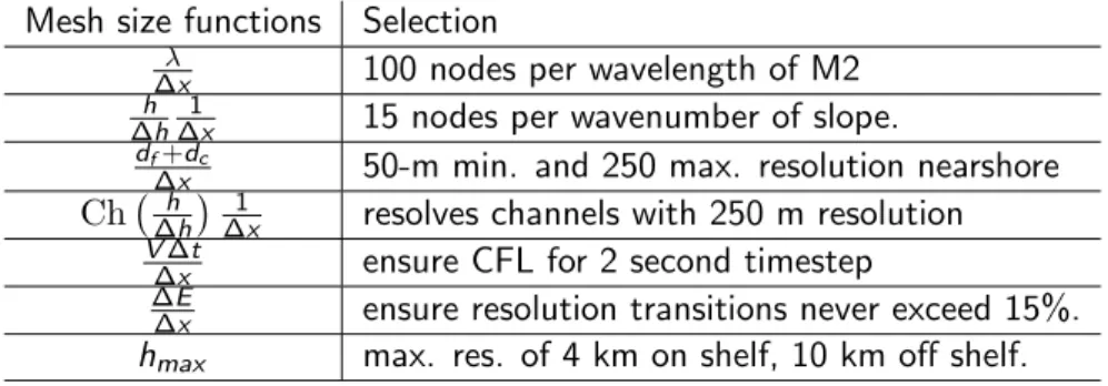
Mesh experiments: Base mesh

I We adopt an experience-based approach to conservatively place mesh resolution so we can later relax it.

Table 2:Mesh size function parameters used to construct the base mesh.

Mesh size functions Selection λ

∆x 100 nodes per wavelength of M2 h

∆h

1

∆x 15 nodes per wavenumber of slope. df+dc

∆x 50-m min. and 250 max. resolution nearshore

Ch _∆h_h_∆1_x resolves channels with 250 m resolution V∆t

∆x ensure CFL for 2 second timestep

∆E

∆x ensure resolution transitions never exceed 15%.

(10)

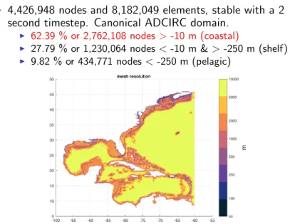
Base mesh: domain

I 4,426,948 nodes and 8,182,049 elements, stable with a 2 second timestep. Canonical ADCIRC domain.

I 62.39 % or 2,762,108 nodes>-10 m (coastal)

I 27.79 % or 1,230,064 nodes<-10 m & >-250 m (shelf)

I 9.82 % or 434,771 nodes<-250 m (pelagic)

(11)

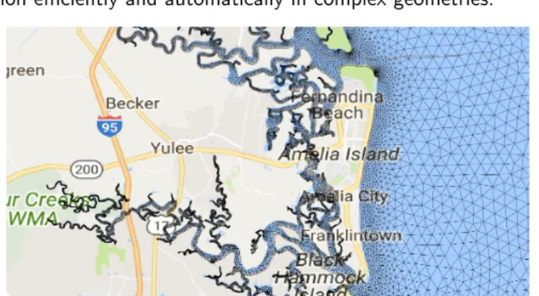
Base mesh feature size

I Boundary representation is identical between mesh resolution experiments (if you aren’t modifying the minimum element size).

(12)

(13)

(14)

Digital elevation data

I Integrating publicly available topobathy datasets from USGS and NOAA onto a common 90-m grid.

I Mesh will only be as good as DEM.

I In areas of overlap, the higher resolution DEM is retained.

I All DEMs are vertically adjusted to LMSL.

Bathymetry on base mesh

SRTM15+

CRM

(15)

Problems with bathymetry

I Some areas need to be augmented with sounding data.

(16)

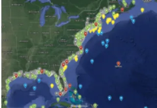
Experimental configuration for tides

I 120 day simulation of tides from Sept. 1-November 31 2012.

I _{DT=2 s, w/ non-linear terms, w/ wetting/drying, IM=511112}

(explicit mass-lumped w/ Smag), Cf=0.0025 (standard quadratic bf coef), NWP=2 (primitive weights, IT coef), TPXO9 constituents on open boundary that spans -60 W from 5 N to 46 N.

I Validating against 421 stations. 1. 379 coastal

2. 25 shelf 3. 17 pelagic

(17)

Base mesh: Tidal validation

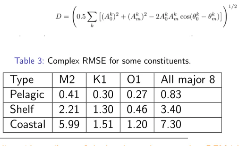
I Calculate the complex RMSE or the discrepancy (D) of either all harmonic constituents or individual ones.

Table 3:Complex RMSE for some constituents.

Type

M2

K1

O1

All major 8

Pelagic

0.41

0.30

0.27

0.83 Shelf

2.21

1.30

0.46

3.40 Coastal

5.99

1.51

1.20

7.30

I Predicts tides well out-of-the box but only as good as DEM is!

(18)

(19)

Base mesh: tidal validation

(20)

Mesh experiments

Does shelf resolution significantly effect predictions of tidal harmonics?

I The representation of the shelf break can be expensive.

I 27% of the mesh (1.2 million nodes) are on the shelf in the base mesh.

I The representation of the shelf break has implications on the calculation of the internal tide coefficient.

C=Cdir

[(N_b2−ω2)( ˜N2−ω2)](1/2) ω

h2_x hxhy

hyhx hy2

(1)

(21)

Mesh experiments

Base→filter slope

h

∆h

1

∆x (2)

Slope/topographic length scale.

I The slope of the bathymetry contains many features that are far smaller than the length scale of the tides.

I Low-pass filter the bathymetry to retain features of comparable length scale to wavelength of M2.

I 825,112 less nodes then base (20% reduction)

(22)

Mesh experiments

Base→filter slope

I Using a 2D gaussian-weighted moving-window averaging filter.2

I In this example, we use a low-pass cutoff length equal to an estimate of the wavelength of the M2 at a reference depth

href of 50 m:

Hwl=

TM2

√

ghref

15 →Hwl=

Hwl

15 (3)

I We divide equation (3) by a constant (15) to get a length scale around 60 km.

1

(23)

Mesh experiments

Base→filter slope

I No significant difference in M2 or K1 amplitude between base and SLPFLT except off the Bahamas bank where the slope feature appears to be critical.

(24)

Mesh experiments

Base→filter slope

I Percent difference

(25)

Mesh experiments

Base→filter slope

(26)

Mesh experiments

Base→filter slope

(27)

Mesh experiments

Base→filter slope

I Regardless, the changes are weak so the RMSE total complex errors don’t change significantly between base and the

SLPFLT (left panel).

(28)

Mesh experiments

Base→filter slope→remove slope, remove bound on shelf

I Since we didn’t see any large scale difference in the harmonics validation, lets further relax the representation of the shelf.

I Remove the 4 km upper bound on shelf resolution and remove the slope mesh size function altogether.

I 235,481 nodes less than SLPFLT (25% less nodes than base).

(29)

Mesh experiments

I Once again, we compare with the base.

I We see generally an even larger amplification of the M2 and K1, especially off the Bahamas and along the Georges bank, but still relatively weak.

(30)

Mesh experiments

I And in percent difference...

(31)

Mesh Experiments

I The coarser representation of the shelf break and shelf features seems to amplify the excursion of the M2.

(32)

Mesh experiments

(33)

Mesh experiments

I But once again, the RMSE total complex errors don’t change significantly from the base solution. (left panel).

(34)

Mesh experiments

Mesh grade relaxation

I Building meshes with slope appears to create percent differences on the order of 5-10%.

I The Georges bank has some non-local effects elsewhere in the Gulf of Maine (albeit 1-3 cm)

I We can further reduce the representation of the shelf, by increasing the relaxation rate or grade of the mesh topology. I 3.36 million nodes → to 2.30 million (34 % reduction in

nodes).

(35)

Mesh grade

Mesh grade relaxation

I While increasing the grade reduces the number of nodes, it further increases the amplification in the Gulf of Maine and along the Bahamas bank.

(36)

Mesh grade

(37)

Mesh grade relaxation

I The shelf station errors becomes worse (1 cm increase) when we relax the grade.

(38)

Summary of results

I As we coarsen the representation of the shelf, a common difference pattern emerges from the base.

(39)

Summary of results

(40)

Summary of results

(41)

Summary of results

(42)

Summary of results

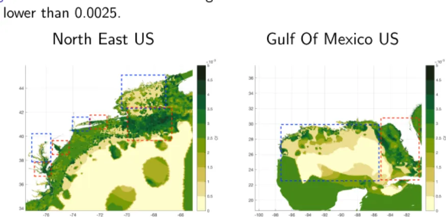
I The pattern of amplification/de-amplification that occurs when the shelf and shelf break are coarsened seems to conform well to our estimation of the Cf bottom friction coefficient.

Figure 4:A red box indicates a Cf greater than 0.0025 and a blue box a Cf lower than 0.0025.

(43)

Conclusions

I We have produced high resolution (min res. 50-m) stable meshes (2 s timestep with non-linear terms) of the entire East Coast Gulf Coast region in a handful of hours (a number of times) from publicly available bathymetric datasets.

I Reducing the resolution in and along the shelf reduces the parameterized dissipation associated with the internal tide.

(44)

Conclusions

I Altering shelf resolution influences the magnitude of the M2 and less so, the K1 on the order of 5-10%.

I The largest change in the tidal solution between the hyper-resolved base mesh and a reduced version originated from altering the mesh grade from 15% to 25%.

I _{Is this due to numerical error or physical representation error?}

Both?

I This resulted in some larger errors (10-25%) on the shelf in the Gulf of Maine but otherwise produced fairly similar coastal errors.