A MIXED BOOLEAN AND DEPOSIT MODEL FOR THE MODELING OF METAL PIGMENTS IN PAINT LAYERS

A MIXED BOOLEAN AND DEPOSIT MODEL FOR THE MODELING OF

METAL PIGMENTS IN PAINT LAYERS

E

C

B

F

¸

W

D

J

Center for Mathematical Morphology, MINES ParisTech, PSL Research University, 35 rue Saint-Honor´e, 77300 Fontainebleau, France

e-mail: [email protected], [email protected], [email protected]

(Received September 11, 2014; revised April 14, 2015; accepted April 15, 2015)

ABSTRACT

Pigments made of metal particles of around 10µm or 20µm produce sparkling effects in paints, due to the specular reflection that occurs at this scale. Overall, the optical aspect of paints depend on the density and distribution in space of the particles. In this work, we model the dispersion of metal particles of size up to 50µm, visible to the eyes, in a paint layer. Making use of optical and scanning electron microscopy (SEM) images, we estimate the dispersion of particles in terms of correlation functions. Particles tend to aggregate into clusters, as shown by the presence of oscillations in the correlation functions. Furthermore, the volume fraction of particles is non-uniform in space. It is highest in the middle of the layer and lowest near the surfaces of the layer. To model this microstructure, we explore two models. The first one is a deposit model where particles fall onto a surface. It is unable to reproduce the observed measurements. We then introduce a “stack” model where clusters are first modeled by a 2D Poisson point process, and a bi-directional deposit model is used to implant particles in each cluster. Good agreement is found with respect to SEM images in terms of correlation functions and density of particles along the layer height.

Keywords: heterogeneous media, optical properties, paints, random microstructure models.

INTRODUCTION

In automotive applications, most paints consist of multi-layered materials, where each layer has a different purpose, ranging from anti-corrosion to visual aspects (D¨ossel, 2008). The overall appearance of paints depends on the paint composition but also on the spatial distribution of particles, most often heterogeneous and multi-scale (Couka et al., 2015). At the largest scales, where geometrical optics apply, metal particles produce specular reflection and sparkling effects. These effects depend on the chemical nature of the particles, their surface roughness, but also on the dispersion of particles and on clustering effects (Dumazet, 2010).

The description of industrial paint layers is a challenging problem. The separation and identification of chemical elements in paint coatings, used to estimate their dispersion in the material, is a complex task (Yanget al., 2010a;b). At the nanometric scale, the effect of pigments on the optical properties has been studied experimentally and compared with effective medium theories (Cummings et al., 1984). More recently, numerical works have been carried out to estimate the effect of the dispersion of pigments in a deposit model (Azzimonti et al., 2013). To represent the material and compute its properties using numerical means, a microstructural model is required.

In other contexts, microstructure models based on hardcore processes have been proposed to forbid the overlap of inclusions in the embedding medium. The effective elasto-plastic response of particle-reinforced composites has been studied in Chawla

et al. (2006), making use of an optimized hardcore procedure to generate microstructures. In Moreaud

et al. (2012), a hardcore deposit model is proposed to simulate a boehmite material. However, the simulation of microstructures using hardcore models becomes difficult when approaching the close-packing limit (Escoda et al., 2015). To overcome this difficulty, random walk stochastic procedures have been developed (Altendorf and Jeulin, 2011) to generate fibrous microstructures, as an improvement on random sequential adsorption models (Feder, 1980). Another problem concerns the generation of multiscale models, for which various methods have been proposed (Paciornik et al., 2002; Jean et al., 2011).

the dispersion, size, shape and orientation of particles using various morphological tools. We introduce and evaluate a deposit and “stack” model, we conclude on their ability to modelize the dispersion of the metallic particles.

METHODS

OPTICAL AND ELECTRON MICROSCOPY IMAGES

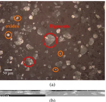
This work focuses on a sparkling, grey-colored industrial paint layer used in automotive applications. The material color results from two types of pigments: several metal oxides of unknown composition, not larger than a few micrometers, and, at a larger scale, aluminium metallic particles of up to 50 µm visible

to the eyes. The two types of pigments are encircled in red and orange respectively in Fig. 1a, an optical microscopy image representing the surface of the layer. The image, however, does not allow one to separate all pigments. Instead, aluminium particles are clearly visible in SEM (scanning electron microscopy) images (Fig. 1b). This image represents a 2D section orthogonal to the surface layer. As shown in the two views, the average shape of the aluminium particles is flat and the particles are often aligned with the layer surface.

The aim of this work is to characterize and model the shape and dispersion of aluminium particles in the paint layer, which produce its sparkling effects. We disregard the oxide pigments entering the paint composition at a smaller scale. Hereafter, we make use of 5 non-overlapping SEM images similar to Fig. 1b to model the aluminium particles spatial distribution.

The actual manufacturing process and exact composition behind this industrial paint is unknown and is therefore not modeled. Instead, we use 3D models with a small number of parameters to mimic the real material. The latter bear no relation with the actual manufacturing process.

SEGMENTATION AND SEPARATION OF PARTICLES

We now segment the aluminium particles from the background in the grey-level SEM images. We also separate individual particles. This step is necessary for computing statistics on particles. The black region at the top of the image, outside of the paint layer, is first segmented by thresholding the images. The threshold value is chosen manually. Furthermore, the paint layer is not exactly aligned with the borders of the SEM

(a)

(b)

Fig. 1.Surface of the paint layer (a) (taken by optical microscopy on a raw surface of the paint), and its slice, orthogonal to the surface (b) (SEM image, taken in SE mode).

images. We identify it with a parallelogram in each image and measure its disorientation with the image borders.

We now apply an area opening of size 20 pixels with a square structural element to remove noise in the image and smoothen the background (Fig. 2b). The resulting image is segmented by an entropy-based automatic thresholding (Otsu, 1979; Fig. 2c).

Some of the aluminium particles have merged because of the low contrast in the gaps located in between two particles that are close to one another. The watershed algorithm is used to separate the particles. Watershed markers are obtained in several steps. We first compute the distance function given by successive erosions using a horizontal structural element (Fig. 2d). The size of the structural elements size is 3 pixels. The deepest markers are extracted from the distance map using the H-maxima algorithm (Schmitt and Preteux, 1986) with size parameter set to 35 pixels. The histogram of the distance map is stretched for more convenience. Using the markers, we compute the watershed partition on the inverse of the distance map previously computed. This leads to a slightly over-segmented image (Fig. 2e). Only about 6 boundaries per image are not well located. We correct them manually.

(a)

(b)

(c)

(d)

(e)

Fig. 2.Original (a) and opened (b) images. Segmented image (c). Distance by erosion using a horizontal structural element (d). Result of the watershed algorithm (e). Magnification; Resolution of the initial image: 1280×77 pixels.

Hereafter we compute the lineic fraction of particles along the height, the correlation functions, a distribution of size and orientations and statistics on particles aggregates. The area fraction, extracted from the segmented images, is about f=hχ(x,y)ix,y=

6.5%.

FRACTION OF PARTICLES ALONG THE HEIGHT

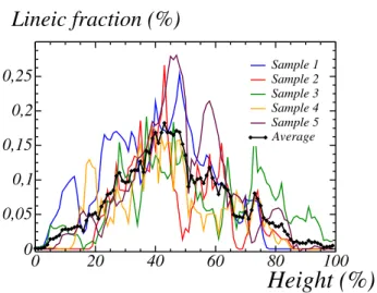
The lineic fraction of aluminium particles is not usually constant along the paint layer height. To estimate it, we first correct the angular deviation of the paint layer in each image by a rotation. The fraction of particles ft(y) =hχ(x,y)ix is then obtained

by averaging over lines parallel to e2 (vertical axis). For each sample, the latter function is represented in Fig. 3 as a function of y/Ly, where Ly is the paint

layer height. We emphasize that this is a relative, not an absolute, distance. The fraction of particles, of about 17%, is highest in the middle of the paint layer, and nearly 0 close to the outer layers. Accordingly, the microstructure is not stationnary in the vertical direction.

0 20 40 60 80 100

Height (%)

0,05 0,1 0,15 0,2 0,25

Lineic fraction (%)

Sample 1 Sample 2 Sample 3 Sample 4 Sample 5 Average

Fig. 3. Lineic fraction of particles along the paint height, for the 5 samples (colored curves) and their mean (black line).

CORRELATION FUNCTION

The covariance function is defined as the probability :

C(r) =P{x∈H,x+r∈H}, (1)

whereH is the union of the aluminium particles, and

x is a point. At large distances |r| 30 µm the two

events x∈H and x+r∈H become uncorrelated andC(r=∞)≈C(0)2_{. Thus, we define the normalized} covariance, or correlation function, as:

C(r) = C(r)−C(0) 2

C(0) [1−C(0)]. (2)

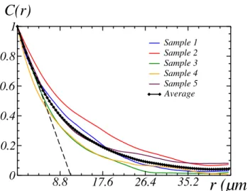
We take r=re1 (r ≥0), aligned with the paint layer surface (Fig. 4) or r = re2 along the paint height (Fig. 5). The slope at the origin forC(re1) is nearly the same for each sample (Fig. 4). The tangent at the origin, represented in the same figure, intersects the r-axis at about r ≈ 12 µm. This value is the

average length of the particles along the directione1. The “average” here is not an average in number (of particles), but in number of chords,i.e., it is weighted by the particles thickness.

Along the layer height, the correlation function

C(re2) instead shows local minima that are typical of repulsion effects in stacks of non-overlapping inclusions (Fig. 5). Here, the tangent at the origin intersects ther-axis at about 3µm, the mean particle

8.8 17.6 26.4 35.2

_{r (µm)}

0.2 0.4 0.6 0.8 1

C(r)

Sample 1 Sample 2 Sample 3 Sample 4 Sample 5 Average

Fig. 4. Correlation function C(re1) along a direction

parallel to the paint surface: each of the 5 samples (colors), mean (black line).

0 4.4 8.8 13.2 17.6 22

_{r (µm)}

0 0.2 0.4 0.6 0.8 1

C(r)

Sample 1 Sample 2 Sample 3 Sample 4 Sample 5 Average

Fig. 5. Correlation function C(re2) along a direction transverse to the paint surface: each of the5samples (colors), mean (black line).

PARTICLES SIZE AND ORIENTATION

In the following, we model aluminium particles as cylinders and measure the distribution of lengths along the principal direction of the particles to infere their size distribution in 3D. We first identify two extremal points in each particle, with maximum and minimum coordinate along e1. The thickness of the particle is estimated as the diameter of the inscribed circle centered in the middle of the two extremal points (Fig. 6). Knowing the centre of each particle, we compute the size of the inscribed circle from the dilation by a rhombicuboctahedron. The orientation and length along the main direction of the particle is estimated by simple geometrical formulae (Fig. 6).

Fig. 6. Representation of the identification of the parameters of a segmented cylinder.

Assume first that all particles are identical cylinders with the same basis diameter D, and unspecified distribution of orientations. The particles appear as elongated rectangles on a 2D section. The cumulative distribution of the lengthL of the largest side of the rectangles reads:

P1(`) =P{L≤`}= 2

πsin −1 `

D . (3)

The cumulative distribution function for the measures is concave whereas it is convex for the theoretical distributionP1(`), as seen in Fig. 7, which invalidates our hypothesis. Therefore, we seek for an alternative 3D model for the particles size distribution.

We notice the existence of small particles in optical images, and consider a uniform distribution of diameters in the range [0;D] for the cylinders basis. The resulting cumulative distribution is derived by integrating on Eq. 3. We find:

P2(`) = 2

π tan

−1_√ `

D2_−`2+

`

Dlog

D+√D2_−`2

`

!

.

(4) Choosing D = 26.4 µm, a good agreement is

0 22 44 66 88

l (µm)

0 0,2 0,4 0,6 0,8 1

P(l)

Uniform radius Constant radius Measures

Fig. 7. Cumulative distribution of the lengths of the particles along their main direction, on a 2D section: measurements (red), theoretical distribution for cylinders with constant (green) or uniform diameter (blue).

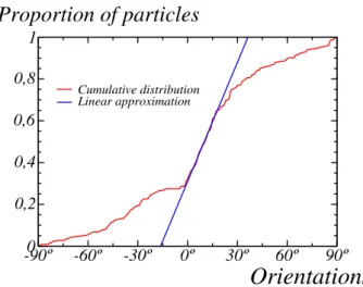
The orientation of the particles, defined as the angle between their main directions and the surface of the paint, is extracted using previously computed points (Fig. 6). The cumulative distribution function (Fig. 8) as a result of a uniform distribution is linear in the range [−3.5◦; 21.5◦]. Many of the misoriented particles are small, for which no apparent orientation is visible. Neglecting the latter, and centering the distribution around 0◦, we model the orientation of the particles as a uniform distribution in the range [−12.5◦; 12.5◦].

-90º -60º -30º 0º 30º 60º 90º

Orientations

0 0,2 0,4 0,6 0,8 1

Proportion of particles

Cumulative distribution Linear approximation

Fig. 8.Cumulative distribution of the orientation of the particles, with respect to the paint layer surface (blue). The latter is quasi-linear in the range [−3.5◦; 21.5◦]

(red).

DISTRIBUTION OF AGGREGATES As seen in SEM images (Fig. 1), particles tend to aggregate in the direction transverse to the surface of the paint layer, as “stacks”. We define stacks as lines transverse to the surface layer and construct them recursively. Each stack initially contains one particle. We identify them with the line passing by the particle center, parallel to the direction e1. We merge two stacks if the distance between them is smaller than the mean radius of all particles, about 7.24µm. Once

again, the new stack is defined as a line transverse to the surface layer. Its e1 coordinate is the average of that of the merged stacks, weigthed by the number of particles each of them contain. The process is stopped when stacks can not be merged anymore. An example of the set of stacks is shown in Fig. 9. The number of particles per stack does not exceed 6. Its statistic is given in Table 1. The mean number of particles per stack is 1.7. Accordingly, the mean distance between two particles in one stack is 5.85µm.

Fig. 9. Distribution of particles along “stacks” (red lines).

Table 1. Proportion of stacks (column 2) per number of particles (column 1).

Particles per stack Proportion of stacks

1 56.9%

2 28.8%

3 7.84%

4 3.27%

5 1.96%

6 1.31%

RESULTS

We compare now the measures obtained on the SEM images to the ones taken on numerical random microstructure models. For the sake of simplicity, we model the particles as cylinders in the rest of this work. Their diameters follow a uniform distribution in the range [0;D] with D=26.4 µm. The angle between

the cylinder basis and the surface follows a uniform distribution as well, in the range [−12.5◦; 12.5◦]. Furthermore, we fix the cylinders’s aspect ratio (basis diameter over height) to 4. This value is consistent with the particles surface density, related to the slopes at the origin of the correlation functions (Figs. 4 and 5).

DEPOSIT MODEL

In this section, we model the dispersion of particles by a 3D deposit model. This model is loosely inspired by the actual fabrication process of the material. Cylinders fall along direction e2 from the top of the simulated domain to the bottom. If they encounter another cylinder, or the bottom, they are moved in the opposite direction, from bottom to top, by a distance

d. Their initial position is taken randomly on the top of the domain. If a cylinder is not entirely contained in the domain, it is rejected and a new initial position is chosen for another cylinder.

The simulation is stopped afterN failed attempts. This number controls the density of particles at the top of the layer. This model has two parameters: the repulsion distance d and the number of failed attempts N. The repulsion distance is chosen as a random variable in the range[0;d_max]to allow contact points between particles as seen in the SEM images (Fig. 1). We choosedmax/2=D/2. This value is close to the mean distance between two particles in a stack (5.85µm). Furthermore, we move cylinders by steps of

2 voxels. This low value is necessary in order to make sure that no cylinder passes through another.

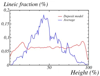
We let N vary to recover the measured surface fraction of particles, and find N =30. A 2D section of the model is represented in Fig. 10. The fraction of particles along lines parallel to the surface layer is represented in Fig. 11 with respect to the height coordinate e2, and compared with that of SEM images. For the deposit model, we average over 100 configurations of size 1024×1024×104 voxels. Although the fraction of particles is 0 along the bottom and top of the model as in the real material, the fraction of particles is overall much more regular in the deposit model than in the paint layer. In the deposit model, the variation of the particle fraction near the surfaces is controlled by the size of the cylinders and their orientation. However, these two parameters are unable to reproduce the fluctuations observed in the SEM images.

Likewise, we compare the model in terms of correlation function (Fig. 12). The slope at the origin is correctly reproduced. Repulsion effects show up as a local minimum on the correlation function for the deposit model around a size of 5.85 µm. This

size is comparable to that of the bump observed on the SEM images. This bump is itself an effect of local minima in the correlation functions of individual samples (Fig. 5). Nevertheless, repulsion effects are much more pronounced in the deposit model than in the paint layer. Thus, both measures investigated here, the fraction of particles along lines parallel to

the surface and the correlation function, invalidate our deposit model. In the next section, we consider a different model where we directly use statistics on the number of particles per stack.

Fig. 10. 2D section of the deposit model. White: particles.

50 100

Height (%)

0,05 0,1 0,15 0,2

Lineic fraction (%)

Deposit model Average

Fig. 11. Mean fraction of particles hχ(x,y)ix as a

function of the height y: SEM images (blue) and deposit model (red).

0 4.4 8.8 13.2 17.6 22

_{r (µm)}

0.2 0.4 0.6 0.8 1

C(r)

Deposit model IEM images

Fig. 12.Correlation functions over 2D sections of the deposit model (red) and SEM images (blue).

STACK MODEL

The validity of this assumption will be examined later on. Second, we associate each stack with a random number of particles. This random number follows the distribution in Tab. 1. Next, particles are recursively added in the simulated domain, along each stack. Each particle is a cylinder with shape, size and orientation defined as in the deposit model. As in the deposit model, the particles do not intersect. Initially, we place the center of each cylinder at a random initial position along the stack axis. This initial position follows a given distribution. Cylinders are moved along the stack axis to the top of the domain if the initial position is closer to the top than it is from the bottom. Otherwise we move the cylinder in the opposite direction. We let the cylinder move as long as it intersects another cylinder.

The distribution of initial positions strongly influences the final density of particles along e2, as computed in Fig. 3. We choose a triangular distribution, symmetrical around the middle of the stack axis. More precisely, we take:

f(y) = 





(1/δ) [1−(1/δ)|y−L2/2|] if |y−L₂/2|<δ

0 otherwise,

(5)

whereL₂is the width of the domain,i.e., the distance between the bottom and top. The density of probability

f(y) is highest at the center y=L2/2 and decreases linearly withy. It is zero aty=L2/2±δ. We optimize

on the parameter δ to approach the density fraction

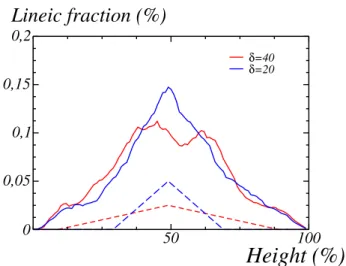
of the SEM images, in terms of least squares. The density fraction of the cylinders in the stack model is narrow for small values ofδ and wider for large values

(Fig. 13). We findδ=0.05L2as optimal value.

Two random 2D sections of the optimal stack model are shown in Fig. 14, together with one segmented SEM image for comparison. Overall, the stack model is much more heterogeneous than the deposit model. On the one hand, particles are stacked together as clusters. On the other hand, isolated particles appear, although no repulsion effect has been introduced in the model. We remark that both features are present in the SEM images. Furthermore, there exists vertical areas joining the bottom and top which are free of particles. This last feature is present in the deposit model but is difficult to control. It presumably has implications on the optical rendering. Hereafter, we compare our model with SEM images in quantitive ways.

50 100

Height (%)

0 0,05 0,1 0,15 0,2

Lineic fraction (%)

δ₌₄₀ δ₌₂₀

Fig. 13. Effect of the parameter δ on the density

fraction of particles in the stack model (over 100

realisations): δ = 20 (blue), δ = 40 (red). Dotted

lines: probability density as defined in Eq. 5, governing the initial position of the cylinders.

The density fraction of particles alonge2is shown in Fig. 15 and compared with measures on the SEM images. Measures for the stack model are averaged over 100 configurations of size 1024×1024×104. As expected, the higher concentration of particles in the middle is recovered in the stack model. Overall, the density fraction of particles is very close to that of the real material.

(a)

(b)

(c)

0 50 100

Height (%)

0,05 0,1 0,15 0,2

Lineic fraction (%)

Stack model IEM images

Fig. 15.Density of particles over lines parallel to the surface layer, as a function of the coordinate along the heighte2: stack model (red), SEM image (blue).

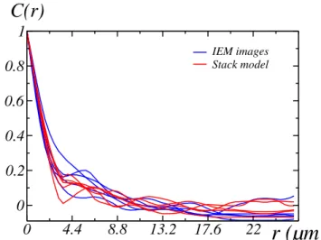
We now evaluate our stack model in terms of the correlation function C(re2) along e2. The correlation functions of individual SEM images show fluctuations characteristic of repulsion effects (Fig. 5) or hardcore phenomena due to contact points in 3D. This effect disappears when averaging the correlation functions measured over all the images of the sample (black curve). Accordingly, we compare separately the correlation functions of one 2D section of random configurations of the stack model with individual SEM images (Fig. 16), and that of averages (Fig. 17). For the latter, we average over all SEM images and over 10 realisations of the 3D stack model. Overall, the correlation functions for the stack model follow the same patterns as in SEM images. Averaging suppresses the fluctuations observed on individual sections for r > 5 µm, for both SEM images and

the stack model. Furthermore, these fluctuations are of the same order of magnitude in the SEM images and 2D sections of the stack model. However, the correlation functions of SEM images show slightly larger differences between individual images than was found for random configurations of the stack model. Good agreement is found between the means of correlation functions as well (Fig. 17): the slopes at the origin are nearly the same, and the correlation functions show a regime change at about 4 µm. The

small discrepancy observed at length scale larger than 4µm is hardly representative, given the small number

of available SEM images.

0 4.4 8.8 13.2 17.6 22

_{r (µm)}

0.2 0.4 0.6 0.8 1

C(r)

IEM images Stack model

Fig. 16.Correlation function C(re2)alonge2along the

height: individual 2D sections of random realizations of the stack model (red) and individual SEM images (blue).

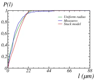
Finally, we compare the distribution of lengths of the particles along their main directions, as observed in 2D sections of the stack model with that of SEM images and the theoretical formula seen in Eq. 4 (Fig. 18). We compute this length by the same methodology as described previously (see Fig. 6). Again, the stack model reproduces the general trend measured on the SEM images.

0 4.4 8.8 13.2 17.6 22

_{r (µm)}

0.2 0.4 0.6 0.8 1

C(r)

Stack model Sample

Fig. 17. Correlation function C(re2) along e2 along

0 22 44 66 88

l (µm)

0,2 0,4 0,6 0,8 1

P(l)

Uniform radius Measures Stack model

Fig. 18.Cumulative distribution function of the length of particles along the main directions as observed on SEM images (blue) and stack model (red). Theoretical formula seen in Eq. 4 shown in green.

DISCUSSION

In this work, we studied micrography images of a paint layer. The 2D distribution of sizes and orientations of metallic particles, measured along sections in the material, were used to determine similar 3D parameters required by the modeling. Furthermore, the dispersion of the particles showed strong clustering effects and inhomogeneous dispersion along the height of the paint layer. The particles density is highest along the middle of the layer and zero along its borders.

A basic deposit model where particles fall along the direction normal to the paint layer was unable to qualitatively reproduce the observed clustering effects and fluctuations of density over the height. Accordingly, we modelled the particles dispersion by a combined Poisson point process for the clusters and a hard-core process for implanting particles in each cluster. We use statistics on the number of particles per cluster and density of clusters in the paint layer, that were determined on the SEM images. The resulting “stack model” showed good agreement with the SEM images in terms of particles size and correlation functions. The density of particles along the height is also well reproduced. This stack model is straightforward to implement and requires only one parameter that is easy to identify. It may also take into account particles with any distribution of shapes and orientations, and could be adapted to other similar paints.

ACKNOWLEDGEMENT

This study was made with the support of A.N.R. (Agence Nationale de la Recherche) under grant 20284 (LIMA project). The authors are grateful to Philippe Porral and Christian Perrot-Minnot (PSA, France) for providing the material samples, and to Mona Ben Achour, Anthony Chesnaud and Alain Thorel (Center of Material, MINES ParisTech, PSL Research University) for contributing images of the material.

REFERENCES

Altendorf H, Jeulin D (2011). Random walk based stochastic modeling of 3D fiber systems. Phys Rev E 83(4):041804.

Azzimonti DF, Willot F, Jeulin D (2013). Optical properties of deposit models for paints: full-fields FFT computations and representative volume element. J Modern Opt 60(7):1-10.

Chawla N, Sidhu R, Ganesh V (2006). Three-dimensional visualization and microstructure-based modeling of deformation in particle-reinforced composites. Acta Mater 54:1541-48.

Cummings KD, Garland JC, Tanner DB (1984). Optical properties of a small-particle composite. Phys Rev B 30(8):4170-82.

Couka E, Willot F, Jeulin D, Ben Achour M, Chesnaud A, Thorel A (2015). Modeling of the multiscale dispersion of nanoparticles in a hematite coating. J Nanosci Nanotech 15(5):3515-21.

D¨ossel KF (2008). Top coats. In: Streitberger HJ, D¨ossel KF, eds. Automotive paints and coatings, 2nd Ed. Weinheim, Germany: Wiley-VCH.

Dumazet S (2010). Mod´elisation de l’apparence visuelle des mat´eriaux – rendu physiquement r´ealiste. PhD thesis, Chtenay-Malabry, ´Ecole centrale de Paris.

Escoda J, Jeulin D, Willot W, Toulemonde C (2015). 3D morphological modeling of concrete using multiscale Poisson polyhedra. J Microsc 258:31–48.

Feder J (1980). Random sequential adsorption. J Theor Biol 87(2):237-54.

Jean A, Jeulin D, Forest S, Cantournet S, N’Guyen F (2011). A multiscale microstructure model of carbon black distribution in rubber. J Microsc 241(3):243-60. Moreaud M, Jeulin D, Morard V, Revel R (2012). TEM

image analysis and modelling: application to boehmite nanoparticles. J Microsc 245(2):186-99.

resin/carbon-black nanocomposites. Eur Phys J Appl Phys 21(1):17-26.

Schmitt M, Preteux F (1986). Un nouvel algorithme en morphologie mathmatique: les r,h maxima et r,h minima. 2i`eme Semaine Internationale de l’Image

´

Electronique 469-475.

Yang S, Gao D, Muster T, Tulloh A, Furman S, Mayo S,

Trinchi A (2010 a). Microstructure of a paint primer – a data-constrained modeling analysis. Mater Sci Forum 656:1686-89.