Oviedo University Press 176 Economics and Business Letters
8(4), 176-190, 2019
Rethinking the financial Kuznets curve in the framework of income
inequality: Empirical evidence on advanced and developing economies
Onur Özdemir*
Istanbul Gelisim University, Department of International Trade (English), Istanbul, Turkey
Received: 8 January 2019 Revised: 4 May 2019 Accepted: 14 May 2019
Abstract
Contrary to the empirical findings that there is a negative link between financial sector development and income inequality, we introduce a different result: in the earlier stages of the financial and economic development, the level of income inequality decreases, but with an ongoing developmental process, the later stages show that the above-mentioned link between finance and inequality turns into positive within the framework of financial Kuznets curve. In terms of finance-inequality nexus, we find that neither markets nor institutions play a significant role for the decrease in income inequality. When the results are measured within this context, the study concludes that the U-shaped financial Kuznets curve hypothesis is valid in the sample countries.
Keywords: Kuznets curve; financial development; income inequality; globalization; U-shape JEL Classification Codes: D31, F01, N20
1. Introduction
The financial sector development and income inequality nexus have already been examined by different perspectives including both orthodox and heterodox knowledge within the categories of advanced and developing economies, yet the common consensus about its causes and reasons is still misleading in the literature. While there are numerous studies that focus on this nexus, the investigation of existing development in finance within the case of financial Kuznets curve is rare1. Financial Kuznets curve is basically used to show that there is an existence of an in-verted U-curve relationship between financial sector development and income inequality. In that token, related to the financial Kuznets curve, three major theoretical papers can be referred to find out the differences of this nexus in the empirical structure. While the first two studies (e.g., Banerjee and Newman, 1993; Galor and Zeira, 1993) argue that making the financial sector more developed leads to lower inequality levels in distributing income among different social segments, the latter (e.g., Greenwood and Jovanovic, 1990) states that there is an inverted
* E-mail: [email protected].
Citation: Özdemir, O. (2019) Rethinking the financial Kuznets curve in the framework of income inequality:
Em-pirical evidence on advanced and developing economies, Economics and Business Letters, 8(4), 176-190.
DOI: 10.17811/ebl.8.4.2019.176-190
1 The major hypothesis of Kuznets curve has been also embraced from different perspectives such as political
U-shaped link for this nexus by indicating that the income inequality increases in the infant
periods of financial development but together with a certain level of financial and economic development, it leads to pursue a lower income inequality.
While these papers are the pioneers of the discussion about the nexus between financial Kuz-nets curve and income inequality, there are also other studies in which they have different pieces of empirical evidence. However, the findings in the following papers differ on the basis of our empirical outcomes due to several reasons. First, Jaumotte et al. (2008) argue that the income inequality has increased over time because of the different reasons (e.g., financial globalization and technological progress) but they shallowly investigate the effect of financial development on inequality by using only depth indicator estimated by the ratio of credit to the private sector by deposit money banks and other financial institutions to GDP. Therefore, they all neglect the effects of the measures of financial access and efficiency which are critical indicators for ana-lyzing income inequality, especially in terms of developed economies. Second, Kappel (2010) backs Banerjee and Newman (1993) and Galor and Zeira (1993) on the basis of empirical evi-dence that the negative relationship between financial development and income inequality is prevailing across different countries. However, Kappel (2010)’s findings are also doubtful due to the data selection in which the paper measures the effect of financial development on ine-quality and poverty by way of using only one indicator for estimating the financial sector de-velopment. Third, Nikoloski (2012) finds that there is an inverted U-curve relationship between financial sector development and income inequality which confirm the theoretical stipulations of Greenwood and Jovanovic (1990). However, the same mistake is done by Nikoloski (2012) in the empirical analysis since the financial sector development is only measured by the credit to private sector and thus overlooks the other critical determinants such as financial system deposits (% of GDP) or bank deposits (% of GDP). There is a potential that Nikoloski (2012)’s inverted U-shaped results may turn into U-curve relations through using these variables. Fi-nally, Tan and Law (2012) and Jauch and Watzka (2016) find similar empirical results as in that paper. While the dataset for income inequality is somewhat similar to those papers, the major difference of this paper depends on the sample selection in which Tan and Law (2012) only examine the dynamics of the finance-inequality nexus in selected developing countries but Jauch and Watzka (2016) extend the sample also by including low-income countries2.
Making analysis for the case of diversifying levels of income inequality across different econ-omies on the basis of financial Kuznets curve hypothesis is important for two reasons. First, the increasing level of income dispersion among different countries can be investigated either with economic indicators and financial indicators in case of short- and long-term periods. Second, the reactions of development stages for financial markets and institutions upon income distri-bution can be well-documented, especially in terms of the classification of different markets.
Several models theoretically utilize the use of private credit over GDP as a proxy variable for financial sector development. In that vein, they ignore the institutional effects of the financial sector on income inequality. Therefore, the market-based use of this kind of proxy indicator stimulates to emerge in two conditions: on the one hand, a higher level of financial development strictly needs human capital which also requires financial credits; on the other hand, the house-holds can access more investment possibilities providing through the financial sector. Rajan (2010) discusses the finance and inequality nexus by looking at political dimensions in the form of redistributive taxation. The main arguments of the study suggest that the financial sector development is highly affected by the political components and depends on increased inequal-ity3. Furthermore, the study provides knowledge that there is a political inability to benefit from
2 For more information about the theoretical discussions please also see Baiardi and Morana (2018).
3 Rajan (2010) provides a better rationale for finance-inequality nexus by incorporating the political dimensions
the traditional implications of redistributive taxation methods. The policy conclusions provide
information that the politicians can have more power to develop new ways for improving access to the financial credits for lower income segments of American households. Similarly, Haan and Sturm (2017) report pieces of empirical evidence which suggest that the level of financial development conditions the impact of financial liberalization on inequality4. Therefore, their results indicate that the alternative channels must be at work that connect finance with income inequality.
Depending to the arguments of above-mentioned three major theoretical studies, the differ-ences at the level of changing knowledge on financial Kuznets curve should be divided from each other, which constitute the basis for further studies, especially in empirical structure. While Banerjee and Newman (1993) work on the mutual relationship between households’ occupa-tional choice dependency and credit availability, Galor and Zeira (1993) focus on human capital investment based on credits. Alternatively, Greenwood and Jovanovic (1990) examine the de-tails of an increasing household capital incomes in the context of financial intermediation and thereby the household portfolio selection process. In the earlier stages of economic develop-ment, the households from the poorer segments of the society cannot be able to use banks for their savings. The financial sector as a whole is almost under-developed and the level of eco-nomic growth is very low. Only the households from the upper-income segments of the society can afford using banks to finance their investments. In that stage, an increase in the level of financial development leads to a higher level of income inequality. Over time, however, the economy develops and the households from the lower-income segments of the society become richer in which they can benefit from financial resources and bank finance. Hence, income inequality begins to decline after a certain point with higher levels of financial and economic development. By extending these models in the direction of both financial markets and institu-tions, it may be possible to have a negative effect of financial sector development on income inequality where the initial results can lose their importance within the frame of different indi-cators such as financial liberalization and labor market policies. So, the U-shaped financial Kuznets curve structure that we are interested in can be different from what the traditional knowledge argues.
Following this manner, three hypotheses on the finance and inequality nexus emerge in which we empirically analyze in the subsequent sections:
Hypothesis 1
There is a long-run positive relationship between financial sector development and income inequality.
Hypothesis 2
There is a positive link between higher levels of openness in financial and trade sectors and more unequal distribution of income.
Hypothesis 3
There is a U-curve relationship between financial and economic development and income inequality.
We re-examine the endogenous relationship between financial sector development and in-come inequality using a panel fixed-effects model and also Generalized Methods of Moments
be checked in empirical framework by which the traditional measures such as private credit to GDP will not be necessary for the generalization of his study in terms of the political dimensions. Therefore, as it is explained in the data part, the financial Sector development data developed by Svirydzenka (2016) will be much proper than that of the traditional variables, which are only focused on depth measures and neglects the Access and efficiency indicators of financial development.
(GMM) for a large sample of countries covering the 1993-2013 period, thereby focusing on
within-country developments of inequality within the framework of financial Kuznets curve. The main rationale to use a fixed-effects panel method is to correct the country-specific effects and thus to remove their correlation with the explanatory variables. Additionally, another ra-tionale is to check the endogeneity problem which may emerge due to omitted variable bias and reverse causality by way of employing GMM procedure developed by Arellano and Bond (1991)5.
As the dependent variable, we use yearly data of Gini coefficients based on the index of ine-quality in equivalized household disposable (i.e., post-tax and post-transfer) income obtained from Solt’s (2016) Standardized World Income Inequality Database (SWIID). Using an index of financial sector development6, including both financial markets and financial institutions, based on the index of Svirydzenka (2016), we find that the income inequality decreases with a higher level of development in the earlier stages of economic and financial conditions but then increases in the future period. Therefore, we reject the theoretical propositions of Greenwood and Jovanovic (1990) for an inverted U-curve relationship between financial sector develop-ment and income inequality.
2. Model and data
To estimate the effect of financial sector development on income inequality, we employ the data of Svirydzenka (2016). The main rationale behind using this variable is to estimate the combined effects of sub-indices for financial markets, financial institutions and overall devel-opment, covering depth, access, and efficiency on income inequality. Therefore, in contrast to the traditional wisdom about the estimation of financial sector development, which is generally conducted for employing credit ratio over GDP, the use of this combined variable is also indi-cated the divergence point of this paper than that of these studies from the traditional wisdom. While this case shows one of the advantages of this study, the other one depends on the fact that this combined data for financial sector development provide a multi-dimensional approach to classify and analyze countries in terms of their financial development through their differ-ences in financial markets and institutions. Related to this information, Svirydzenka (2016: 4) argues that the constellation of financial institutions and markets facilitates the provision of financial services. Therefore, the exclusion of their sub-components (e.g., depth and access) from the estimation process provides a limited understanding of the finance-inequality nexus. An important characteristic of financial systems over the advanced and developing economies is their having to a higher level of access and efficiency as well as the higher level of depth. The differences in financial systems across these countries imply that multiple indicators are needed to measure financial development (Čihák et al., 2012; Aizenman, Jinjarak and Park, 2015). To overcome these problems, which root in using single indicators as proxies for finan-cial development, we add this data provided by Svirydzenka (2016) which is culminated in the overall index of financial development. In that vein, the data is measured on a ratio between 0 to 1 (fully underdeveloped to fully developed)7. Our first measure of the financial sector devel-opment is estimated as the weighted average of both financial markets and institutions indices.
5 For more information about the empirical approach please see Part 3.
6 We separately use the data of financial markets and financial markets in the models to extend the analytical
framework economically and institutionally in terms of financial sector as a whole.
7 Financial institutions (FI) index measures access to financial institutions, efficiency of these institutions (interest
As these indices about the financial sector development are not widely used in the literature
upon the financial Kuznets curve, we exert an additional proxy variable which is private credit by deposit money banks to GDP in order to catch the difference from other studies such as Greenwood and Jovanovic (1990), Banerjee and Newman (1993) and Galor and Zeira (1993). Our sample for which we use the indices of financial sector development and additional proxy variable for measuring financial development in case of financial depth consists of 61 countries8 (including both advanced and developing economies) and runs from 1993 to 2013.
In addition, the independent variables include the globalization indices obtained from KOF Index of Globalization and openness measures including trade openness and capital account openness obtained from World Development Indicators (WDI) and Chinn and Ito (2006), re-spectively. First, KOF Globalization Index, which is provided by Gygli, Haelg and Sturm (2018), measures the economic, social and political dimensions of globalization. Alternatively, we replace the globalization indices with the openness measures. Second, we, therefore, employ some critical openness measures. On the one hand, to estimate the effect of liberalization in trade, we use real trade openness index estimated by the total of exports and imports divided by GDP which is adjusted from the price of GDP. On the other hand, to test the effects of financial liberalization on income inequality, we employ the Chinn-Ito index (i.e., the KAOPEN index), which handles the capital account openness. The KAOPEN index is a special one compared to the other indices based on financial liberalization in which it grounds on in-formation about the capital mobility obtained from IMF’s Annual Report on Exchange Ar-rangements and Exchange Restrictions (AREAER) to incorporate the extent and intensity of capital controls. Therefore, this index can be evaluated as a de jure measure of capital account liberalization where cannot lead to higher cross-border transactions although the restrictions on these transactions are to a large extent being reduced for both domestic and international capi-tals.
Our dependent variable is the Gini coefficient based on the index of inequality in equivalized household disposable income obtained from Solt (2016)’s SWIID. The database is measured on a gross and on a net basis. Related to this, we use the index that stands for gross household income, which is not adjusted from taxes. As Haan, Pleninger and Sturm (2018: 314) state that this shows income inequality exclusive of fiscal policy. Since the household income is repre-sented both as gross9 and net forms, SWIID has special importance compared to other inequal-ity measures. The Gini coefficient is ranged between 0 and 100. 0 represents perfect equalinequal-ity and 100 represents perfect inequality. Besides the SWIID, income inequality can also be meas-ured by other methods such as dividing income categories from lowest to upper segments of the society. However, the comprehensive database, especially in terms of panel data analysis, is misleading and some years for middle-income countries are missing. Hence, it makes the panel data structure as an unbalanced. In that sense, we take yearly averages of the Gini coeffi-cient from 1993 to 2013 for both advanced and developing economies. In Figure 1, we graph the trends of measures covering both finance and inequality for advanced and developing econ-omies. The left side shows the variables for financial development, while right-side shows the change in income inequality over time.
8 The major reason for choosing these countries is due to the fact that the econometric method that we used in the
empirical part is theoretically grounded on the basis of a balanced panel. Therefore, the data for financial Sector development and income inequality is missing for the rest of the countries.
9 Gross household income excludes non-private series of income and does not give an equal amount of what an
Figure 1. Trends in financial development and income inequality.
Source: Solt (2016), Svirydzenka (2016)
Using panel data from 1993 to 2013, on the one hand, we are interested in the within-country relationship between financial sector development and income inequality tested by fixed-effects method depending on Driscoll and Kraay (1998)’s robust standard error estimator; on the other hand, GMM estimator is employed to examine dynamic changes and to control endogeneity issues. The model is estimated by
GINIi,t = αi + β1FINi,t + β2FIN2i,t + β3FLi,t + β4TLi,t + β5GDPi,t + β6GDP2i,t + βjXi,t + εi,t (1) where GINI is income inequality, FIN consists of all financial development indices and FIN2 is their squared terms, FL is financial liberalization, TL is trade liberalization, GDP is per capita income and GDP2 is its squared term and X is a vector of control variables for globalization indices, unemployment rate, general government expenditure, human capital, and real effective exchange rate whereas ε denotes the error term. Following the hypothesis 1 of linear negative effect, β1 should be negative and significant, and β2 should be positive but also significant. According to our U-shaped hypothesis, these correlations should be done in control of other variables both for proxy variables and sub-indices of financial development. Therefore, we also add liberalization indicators into the regressions, covering both capital account and trade re-gime, and the GDP per capita with its squared term for robustness issues to control for tradi-tional knowledge about the financial Kuznets hypothesis. Interestingly, in accordance with our hypotheses, the β5 should be negative and significant, and β6 should be positive and statistically significant in contrast to the mainstream vision of the Kuznets curve.
We follow the approach of the earlier studies by using the same specifications with different control variables and the OLS method in fixed-effects estimations. Employing our comprehen-sive database lead us to argue that the empirical results for the effect of Fin_Dev, Fin_Ins_Dev, Fin_Mar_Dev, Prv_Cred, Fin_Lib, Trade_Lib and Log GDP on income inequality are signifi-cantly different from the traditional findings and thus frustrates to other studies for the finance and inequality nexus to a certain degree. A summary of the sources for data is provided in Table 1. Additionally, Table 2 presents selected descriptive statistics for selected countries having different income-levels in our sample.
34,4 34,6 34,8 35 35,2 35,4 35,6 35,8 36 36,2 36,4
20 25 30 35 40 45 50 55 60 65
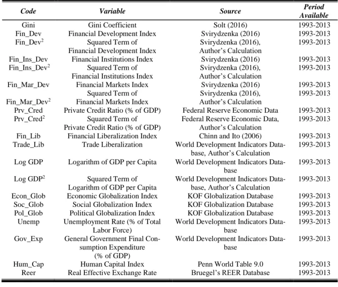
Table 1. Summary of data sources.
Code Variable Source Period
Available
Gini Gini Coefficient Solt (2016) 1993-2013
Fin_Dev Financial Development Index Svirydzenka (2016) 1993-2013
Fin_Dev2 Squared Term of
Financial Development Index
Svirydzenka (2016),
Author’s Calculation 1993-2013
Fin_Ins_Dev Financial Institutions Index Svirydzenka (2016) 1993-2013
Fin_Ins_Dev2 Squared Term of
Financial Institutions Index
Svirydzenka (2016),
Author’s Calculation 1993-2013
Fin_Mar_Dev Financial Markets Index Svirydzenka (2016) 1993-2013
Fin_Mar_Dev2
Squared Term of Financial Markets Index
Svirydzenka (2016),
Author’s Calculation 1993-2013
Prv_Cred Private Credit Ratio (% of GDP) Federal Reserve Economic Data 1993-2013
Prv_Cred2 Squared Term of
Private Credit Ratio (% of GDP)
Federal Reserve Economic Data, Author’s Calculation
1993-2013
Fin_Lib Financial Liberalization Index Chinn and Ito (2006) 1993-2013
Trade_Lib Trade Liberalization World Development Indicators
Data-base, Author’s Calculation 1993-2013
Log GDP Logarithm of GDP per Capita World Development Indicators
Data-base
1993-2013
Log GDP2 Squared Term of
Logarithm of GDP per Capita
World Development Indicators Data-base, Author’s Calculation
1993-2013
Econ_Glob Economic Globalization Index KOF Globalization Database 1993-2013
Soc_Glob Social Globalization Index KOF Globalization Database 1993-2013
Pol_Glob Political Globalization Index KOF Globalization Database 1993-2013
Unemp Unemployment Rate (% of Total
Labor Force)
World Development Indicators Data-base
1993-2013
Gov_Exp General Government Final
Con-sumption Expenditure (% of GDP)
World Development Indicators Data-base
1993-2013
Hum_Cap Human Capital Index Penn World Table 9.0 1993-2013
Reer Real Effective Exchange Rate Bruegel’s REER Database 1993-2013
3. The empirical results
Table 3 and Table 4 include the baseline empirical results of the article. In models (1)-(8), we alternatively use indices on financial development to check the effects of financial sector de-velopment on income inequality in the fixed-effects panel model and GMM technique, respec-tively. While the fixed-effects panel model uses within estimator, we test this relationship with the same variables in control of GMM estimator to avoid endogeneity problem. In other words, we also do these predictions for GMM estimator in case of possibility for endogeneity that the OLS methods can have through taking two lags of Gini coefficient. Since our finance measures may have differential effects on inequality in terms of both markets and institutions, we separate the overall financial development variable from the others. In the next step, we add a traditional indicator for finance as a proxy variable, which is private credit over GDP, to check the diver-sion of our estimation from other empirical findings based on mainstream knowledge.
N panels, (iii) independent variables that are not strictly exogenous, (iv) arbitrarily distributed
fixed-effects, (v) heteroskedasticity, and (vi) autocorrelation within panels. Table 3. Fixed-Effects Panel Model (dependent variable: Gini coefficient).
(1) (2) (3) (4) (5) (6) (7) (8)
Fin_Dev -3.936 -5.726** (2.944) (2.536) Fin_Dev2 4.629* 5.947***
(2.484) (2.014)
Fin_Ins_Dev. -9.244*** -11.907*** (2.947) (3.196)
Fin_Ins_Dev2 6.467*** 8.360***
(2.088) (2.021)
Fin_Mar_Dev. -0.780 -1.107
(1.145) (0.908)
Fin_Mar_Dev2 2.570** 2.896***
(1.074) (0.682)
Prv_Cred -0.006 -0.006
(0.005) (0.004)
Prv_Cred2 0.000** 0.000***
(0.000) (0.000)
Fin_Lib 0.145** 0.146** 0.131*** 0.123***
(0.054) (0.053) (0.042) (0.042)
Trade_Lib 0.734*** 0.668*** 0.807*** 0.688*
(0.253) (0.196) (0.269) (0.340)
Log GDP -0.490 -1.692 0.636 -0.053 -0.865 -2.420 -1.074 -2.349 (3.616) (3.502) (3.660) (3.481) (3.498) (3.515) (3.732) (3.870) Log GDP2 138.311* 145.029* 142.404* 147.271* 125.245 130.914 128.313 128.467 (76.631) (81.397) (70.940) (70.639) (78.599) (83.475) (76.233) (82.856)
Econ_Glob 0.024*** 0.031*** 0.023*** 0.017***
(0.005) (0.008) (0.004) (0.004)
Soc_Glob 0.031 0.037** 0.025 0.025
(0.019) (0.016) (0.021) (0.020)
Pol_Glob -0.006 -0.006 -0.003 -0.007
(0.008) (0.009) (0.008) (0.009)
Unemp 0.135*** 0.136*** 0.108*** 0.105*** 0.140*** 0.144*** 0.117*** 0.121*** (0.014) (0.014) (0.015) (0.016) (0.014) (0.016) (0.014) (0.015) Gov_Exp -0.037 -0.046** -0.030 -0.038** -0.030 -0.034* -0.034 -0.042* (0.023) (0.020) (0.018) (0.014) (0.022) (0.018) (0.023) (0.021) Hum_Cap -4.588*** -4.926*** -4.551*** -4.891*** -4.615*** -5.083*** -4.838*** -5.222***
(0.402) (0.357) (0.387) (0.317) (0.414) (0.382) (0.427) (0.421) Reer 0.005** 0.006** 0.006** 0.006** 0.005** 0.006** 0.005** 0.007***
(0.002) (0.002) (0.002) (0.002) (0.002) (0.002) (0.002) (0.002) Constant 48.552*** 47.258*** 50.965*** 48.891*** 47.481*** 46.226*** 48.973*** 48.228***
(1.405) (1.852) (1.855) (1.937) (1.147) (1.671) (1.479) (1.659) R-squared 0.1693 0.1725 0.1889 0.2042 0.1758 0.1751 0.1660 0.1667 F-test on indices 1096.11 1393.05 1877.76 438.50 834.64 1231.31
F-test on Prv_Cred 3547.82 8648.98
No. of observations 1,281 1,281 1,281 1,281 1,281 1,281 1,281 1,281
No. of countries 61 61 61 61 61 61 61 61
Note. Robust standard errors in parentheses *** p<0.01, ** p<0.05, * p<0.1
estimations consistent. Since our dataset is designed for many panels and few periods and also
the idiosyncratic errors have no autocorrelation, this GMM estimator is robust to our panels. Furthermore, Arellano and Bond (1991) suggest the use of AR(2) test so as to control whether the second-order serial correlation of the error term exists and indicate the significance of Han-sen (1982) J-test to detect whether the orthogonality conditions prevail. Both estimation results show that there is no further serial correlation and the over-identifying restrictions are not re-jected to the degree of Hansen J-test.
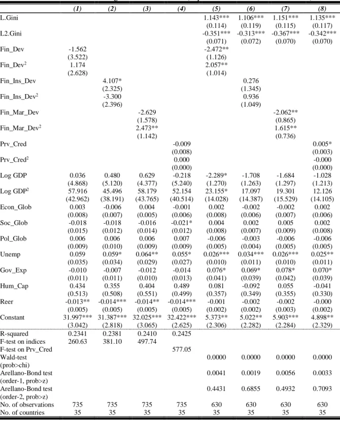
Table 4. Dynamic Panel Model (dependent variable: Gini coefficient).
(1) (2) (3) (4) (5) (6) (7) (8)
L.Gini 1.048*** 1.048*** 1.037*** 1.036*** 1.070*** 1.068*** 1.044*** 1.031*** (0.082) (0.080) (0.077) (0.075) (0.080) (0.079) (0.080) (0.076) L2.Gini -0.253*** -0.242*** -0.244*** -0.235*** -0.274*** -0.260*** -0.249*** -0.228***
(0.069) (0.064) (0.066) (0.062) (0.068) (0.065) (0.069) (0.064) Fin_Dev -1.844** -2.306**
(0.923) (1.040) Fin_Dev2 2.049*** 2.204***
(0.713) (0.801)
Fin_Ins_Dev -2.330** -2.637**
(1.091) (1.146)
Fin_Ins_Dev2 2.440*** 2.456***
(0.854) (0.908)
Fin_Mar_Dev -0.588 -0.932
(0.575) (0.641)
Fin_Mar_Dev2 0.869* 1.072*
(0.499) (0.564)
Prv_Cred 0.008* 0.008*
(0.004) (0.004)
Prv_Cred2 -0.000 -0.000
(0.000) (0.000)
Fin_Lib 0.011 0.011 -0.003 -0.008
(0.034) (0.034) (0.033) (0.033)
Trade_Lib 0.516** 0.517** 0.564** 0.486**
(0.228) (0.222) (0.239) (0.229)
Log GDP -0.372 -0.401 -0.159 -0.211 -0.373 -0.367 0.807 0.855 (0.741) (0.787) (0.725) (0.764) (0.742) (0.789) (0.801) (0.831) Log GDP2 29.505* 26.579 31.074* 28.230* 26.537* 24.103 15.748 13.490 (16.722) (16.900) (16.421) (16.937) (15.191) (15.663) (15.261) (15.490)
Econ_Glob 0.004 0.006 0.002 0.002
(0.006) (0.006) (0.006) (0.005)
Soc_Glob -0.004 -0.004 -0.007 -0.010*
(0.005) (0.004) (0.005) (0.005)
Pol_Glob -0.016*** -0.015*** -0.017*** -0.014***
(0.005) (0.005) (0.005) (0.005)
Unemp 0.019 0.020 0.019 0.021 0.018 0.021 0.018 0.020 (0.013) (0.013) (0.013) (0.013) (0.012) (0.013) (0.013) (0.014) Gov_Exp 0.036** 0.040*** 0.032** 0.034*** 0.040*** 0.044*** 0.031** 0.034** (0.014) (0.014) (0.013) (0.013) (0.015) (0.014) (0.014) (0.014) Hum_Cap -1.469*** -1.525*** -1.511*** -1.558*** -1.528*** -1.565*** -1.465*** -1.495***
(0.484) (0.563) (0.502) (0.570) (0.494) (0.587) (0.473) (0.553) Reer 0.000 0.001 0.001 0.002 0.000 0.001 0.000 0.001
(0.001) (0.001) (0.001) (0.001) (0.001) (0.001) (0.001) (0.001) Constant 10.677*** 11.848*** 10.978*** 12.066*** 10.462*** 11.836*** 10.119*** 11.512***
(2.019) (2.065) (1.967) (2.058) (2.157) (2.174) (2.062) (2.090) Wald-test (prob>chi) 0.0000 0.0000 0.0000 0.0000 0.0000 0.0000 0.0000 0.0000 Arellano-Bond test
(order-1, prob>z)
0.0002 0.0001 0.0002 0.0001 0.0002 0.0001 0.0004 0.0002
Arellano-Bond test (order-2, prob>z)
0.8144 0.8444 0.7745 0.8231 0.8177 0.8405 0.7304 0.7368
No. of observations 1,098 1,098 1,098 1,098 1,098 1,098 1,098 1,098
No. of countries 61 61 61 61 61 61 61 61
However, there are also some limitations of our empirical approach on the basis of both
fixed-effects and GMM estimations. While the fixed-fixed-effects method does not solve the endogeneity problem, the GMM procedure developed by Arellano and Bond (1991) does not find proper solutions to the problems emerging due to the number of instruments. Therefore, further studies will also employ Roodman (2009)’s method in the same models by considering both system-GMM with one- and two-step estimator and collapsing instruments options. These further esti-mations will also compare the empirical evidence produced by difference-GMM and system-GMM procedures.
Table 5. Robustness Checks for High-Income Countries (dependent variable: Gini coefficient).
(1) (2) (3) (4) (5) (6) (7) (8)
L.Gini 1.143*** 1.106*** 1.151*** 1.135***
(0.114) (0.119) (0.115) (0.117)
L2.Gini -0.351*** -0.313*** -0.367*** -0.342***
(0.071) (0.072) (0.070) (0.070)
Fin_Dev -1.562 -2.472**
(3.522) (1.126)
Fin_Dev2 1.174 2.057**
(2.628) (1.014)
Fin_Ins_Dev 4.107* 0.276
(2.325) (1.345)
Fin_Ins_Dev2 -3.300 0.936
(2.396) (1.049)
Fin_Mar_Dev -2.629 -2.062**
(1.578) (0.865)
Fin_Mar_Dev2 2.473** 1.615**
(1.142) (0.736)
Prv_Cred -0.009 0.005*
(0.008) (0.003)
Prv_Cred2 0.000 -0.000
(0.000) (0.000)
Log GDP 0.036 0.480 0.629 -0.218 -2.289* -1.708 -1.684 -1.028 (4.868) (5.120) (4.377) (5.240) (1.270) (1.263) (1.297) (1.213) Log GDP2 57.916 45.496 58.179 52.154 23.155* 17.097 19.301 12.126 (42.962) (38.191) (43.765) (40.514) (14.028) (14.387) (15.529) (14.105) Econ_Glob 0.003 -0.006 0.004 -0.001 0.002 -0.002 -0.002 0.002
(0.008) (0.007) (0.005) (0.006) (0.008) (0.006) (0.007) (0.006) Soc_Glob -0.018 -0.018 -0.016 -0.021* 0.004 0.002 0.005 0.002
(0.015) (0.012) (0.014) (0.012) (0.008) (0.007) (0.009) (0.008) Pol_Glob 0.006 0.006 0.006 0.007 -0.006 -0.003 -0.006 -0.006
(0.009) (0.010) (0.009) (0.009) (0.005) (0.004) (0.005) (0.005) Unemp 0.059 0.059* 0.064** 0.055* 0.026*** 0.034*** 0.026*** 0.025** (0.035) (0.034) (0.029) (0.027) (0.010) (0.011) (0.010) (0.011) Gov_Exp -0.010 -0.007 -0.012 -0.014 0.076* 0.069* 0.078* 0.070* (0.011) (0.011) (0.010) (0.013) (0.041) (0.039) (0.042) (0.039) Hum_Cap 0.434 0.355 0.404 0.489 0.081 -0.092 0.055 -0.041
(0.513) (0.508) (0.551) (0.499) (0.357) (0.349) (0.355) (0.330) Reer -0.013** -0.014*** -0.014** -0.014*** -0.001 -0.002 -0.002 -0.000
(0.005) (0.005) (0.005) (0.005) (0.002) (0.002) (0.003) (0.002) Constant 31.997*** 31.387*** 32.025*** 32.422*** 5.373** 5.022** 5.903*** 4.898** (3.042) (2.818) (3.065) (2.625) (2.306) (2.282) (2.284) (2.329) R-squared 0.2341 0.2381 0.2410 0.2425
F-test on indices 260.63 381.10 497.74
F-test on Prv_Cred 577.05
Wald-test (prob>chi)
0.0000 0.0000 0.0000 0.0000
Arellano-Bond test (order-1, prob>z)
0.0041 0.0019 0.0056 0.0033
Arellano-Bond test (order-2, prob>z)
0.4431 0.6855 0.4932 0.7093
No. of observations 735 735 735 735 630 630 630 630
No. of countries 35 35 35 35 35 35 35 35
The empirical results suggest that measures on financial sector development increase income
inequality in the later stages of economic development while decrease it in the infant period of financial and economic development, irrespective of whether the indices for financial sector development are included separately. This is contradicted to the findings of Greenwood and Jovanovic (1990), Banerjee and Newman (1993) and Galor and Zeira (1993). In control of the endogeneity problem, the results are still relevant and statistically significant. While the reasons for this U-shaped curve for the relationship between finance-inequality nexus, some of the fac-tors can briefly be ranged as follows: (i) the degree of openness to trade and financial accounts, (ii) the differences in the level of economic development, and (iii) the diversity of globalization parameters including both economic, social and political dimensions.
Next, we turn to the estimation of traditional Kuznets hypothesis in which the results are sim-ilar to that of financial Kuznets hypothesis. There is consistency among the variables used for financial sector development. Therefore, the econometric outcomes indicate that financial sec-tor development is conditioned on different facsec-tors for different economies. In that vein, the mainstream arguments in favor of the implementation of pro-liberal policies should consider the reasons for the fluctuations in the degree of income inequality which depend on several issues the economies have to solve in the long-run instead of carrying out a higher level of economic liberalization. In other words, contrary to the mainstream views for more developed finance to provide an equal income distribution among individuals, the countries should follow older strategies in line with the economic and financial development. This conclusion also holds for the measures of openness in trade regime and financial accounts.
We also make further analysis by dividing countries into two categories in terms of their in-come levels so as to understand whether the U-shaped curve relationship between financial sector development and income inequality significantly changes. The following models in Ta-ble 5 and TaTa-ble 6 use the same econometric procedures as in the previous models, which con-sider both fixed-effects and dynamic estimations. However, the empirical results are somehow different from the baseline results. First, the U-shaped link is mostly insignificant for the models (1)-(4) in Table 5 for high-income countries10. Second, the GMM estimations are more reliable than that of the fixed-effects due to their control for potential endogeneity problem. In that vein, the estimation results in the Model (5) and Model (7) are still highly significantly significant and validate the U-shaped curve relationship between financial sector development and income inequality. Additionally, in each regression, there is a high persistence of Gini coefficient and thus the dynamic panel results are much reliable than the static models.
Finally, we also apply the same econometric procedures for middle-income countries in Ta-ble 6, covering both upper- and lower-middle income groups. Unlike the case for high-income countries, the results for the empirical estimations in terms of middle-income countries are striking due to the fact that almost all regression produces a U-shaped curve relationship for financial development-inequality nexus. Therefore, these empirical outputs lead us to argue that the U-shaped linkage is more strong in middle-income countries. All in all, both baseline and sensitivity analyses contradict with the traditional wisdom which finds an inverted U-shaped curve and thus need to be much attention for further estimations.
4. Concluding remarks
Given this background, we test theoretical models, which explain the finance and inequality nexus and which infer that higher levels of financial sector development lead to an increasing level of income inequality. Regarding the income segregations in the society as a whole the inequality level of income decreases in the earlier stages of financial and economic develop-ment but in the later stages, following an increase in aggregate income, the income gap
Table 6. Robustness Checks for Middle-Income Countries (dependent variable: Gini coefficient).
(1) (2) (3) (4) (5) (6) (7) (8)
L.Gini 1.186*** 1.192*** 1.184*** 1.168***
(0.101) (0.097) (0.101) (0.097)
L2.Gini -0.329*** -0.331*** -0.329*** -0.309***
(0.081) (0.079) (0.081) (0.078)
Fin_Dev -12.130*** 1.153
(2.162) (1.775)
Fin_Dev2 17.369*** -1.379
(2.699) (2.704)
Fin_Ins_Dev -18.391*** 1.659
(3.459) (1.503)
Fin_Ins_Dev2 16.580*** -2.070
(2.443) (2.434)
Fin_Mar_Dev -3.784** 0.042
(1.728) (0.682)
Fin_Mar_Dev2 8.623*** 0.056
(1.753) (0.814)
Prv_Cred -0.049** 0.010*
(0.022) (0.005)
Prv_Cred2 0.000** -0.000
(0.000) (0.000)
Log GDP 3.539 6.668 2.133 5.932 1.452 1.269 1.418 1.602 (3.621) (3.966) (3.778) (3.825) (0.980) (0.979) (0.979) (1.098) Log GDP2 208.055*** 224.411*** 176.077** 165.730** 23.074 20.318 24.394 25.502 (51.335) (57.542) (62.786) (59.679) (26.119) (25.474) (25.897) (25.317) Econ_Glob 0.029** 0.027** 0.028*** 0.042*** 0.005 0.005 0.005 0.002
(0.011) (0.011) (0.009) (0.012) (0.008) (0.008) (0.008) (0.008) Soc_Glob 0.097*** 0.106*** 0.083*** 0.086*** 0.002 0.002 0.004 0.001
(0.022) (0.020) (0.024) (0.019) (0.008) (0.007) (0.007) (0.007) Pol_Glob -0.020* -0.016* -0.013 -0.012 -0.015** -0.015** -0.016** -0.016**
(0.010) (0.009) (0.010) (0.010) (0.007) (0.007) (0.007) (0.007) Unemp 0.181*** 0.161*** 0.188*** 0.186*** 0.011 0.009 0.009 0.013
(0.055) (0.041) (0.057) (0.045) (0.022) (0.025) (0.024) (0.025) Gov_Exp -0.062 -0.058 -0.029 0.015 0.014 0.015 0.014 0.011
(0.051) (0.037) (0.049) (0.038) (0.017) (0.016) (0.017) (0.016) Hum_Cap -10.509*** -11.324*** -10.164*** -9.313*** -0.711 -0.474 -0.803 -0.585
(1.056) (0.919) (1.279) (0.864) (0.780) (0.646) (0.736) (0.721) Reer 0.007** 0.008*** 0.007*** 0.010** 0.001 0.001 0.001 0.000
(0.003) (0.003) (0.002) (0.003) (0.002) (0.002) (0.002) (0.002) Constant 64.867*** 68.657*** 61.839*** 58.858*** 8.076** 7.216** 8.540** 7.958** (2.666) (3.119) (2.790) (1.723) (3.608) (2.848) (3.433) (3.297) R-squared 0.3278 0.3702 0.3253 0.3522
F-test on indices 6182.18 1497.07 1682.22
F-test on Prv_Cred 921.66
Wald-test (prob>chi)
0.0000 0.0000 0.0000 0.0000
Arellano-Bond test (order-1, prob>z)
0.0119 0.0115 0.0124 0.0127
Arellano-Bond test (order-2, prob>z)
0.8161 0.7888 0.8312 0.8486
No. of observations 546 546 546 546 468 468 468 468
No. of countries 26 26 26 26 26 26 26 26
Note: Robust standard errors in parentheses *** p<0.01, ** p<0.05, * p<0.1
conditions on increased levels of income inequality. However, we have to point on to the case
that this relationship can change if the openness and financial sector development indicators are treated as interactively, as Haan, Pleninger and Sturm (2018) suggest. Therefore, the results should be evaluated in caution and should be analyzed within different socio-economic and political forms.
References
Aizenman, J., Jinjarak, Y., and Park, D. (2015) Financial Development and Output Growth in Developing Asia and Latin America: A Comparative Sectoral Analysis, NBER Working Pa-per 20917, National Bureau of Economic Research, Cambridge, Massachusetts.
Arellano, M., and Bond, S. R. (1991) Some Tests of Specification for Panel Data: Monte Carlo Evidence and an Application to Employment Equations, Review of Economic Studies, 58, 277-297.
Baiardi, D., and Morana, C. (2018) Financial Development and Income Distribution Inequality in the Euro Area, Economic Modelling, 70, 40-55.
Banerjee, A. V., and Newman, A. F. (1993) Occupational Choice and the Process of Develop-ment, Journal of Political Economy, 101, 274-298.
Bumann, S., and Lensink, R. (2016) Capital Account Liberalization and Income Inequality, Journal of International Money and Finance, 61, 143-162.
Chinn, M. D., and Ito, H. (2006) What Matters for Financial Development? Capital Controls, Institutions, and Interactions, Journal of Development Economics, 81, 163-192.
Chong, A. (2004) Inequality, Democracy, and Persistence: Is There a Political Kuznets Curve?, Economics & Politics, 16, 189-212.
Čihák, M., Demirgüç-Kunt, A., Feyen, E., and Levine, R. (2012) Benchmarking Financial Development Around the World, World Bank Policy Research Working Paper 6175, World Bank, Washington, DC.
Driscoll, J. C., and Kraay, A. C. (1998) Consistent Covariance Matrix Estimation with Spatially Dependent Panel Data, Review of Economics and Statistics, 80, 549-560.
de Haan, J., and Sturm, J.-E. (2017) Finance and Income Inequality: A Review and New Evi-dence, European Journal of Political Economy, 50, 171-195.
de Haan, J., Pleninger, R,. and Sturm, J.-E. (2018) Does the Impact of Financial Liberalization on Income Inequality Depend on Financial Development? Some New Evidence, Applied Economic Letters, 25, 313-316.
Galor, O., and Zeira, J. (1993) Income Distribution and Macroeconomics, Review of Economic Studies, 60, 35-52.
Greenwood, J., and Jovanovic, B. (1990) Financial Development, Growth, and the Distribution of Income, Journal of Political Economy, 98, 1076-1107.
Gygli, S., Haelg, F., and Sturm, J.-E. (2018) The KOF Globalization Index-Revisited, KOF Swiss Economic Institute Working Paper No.439.
Hansen, L. P. (1982) Large Sample Properties of Generalized Method of Moments Estimators, Econometrica, 50, 1029-1054.
Jalil, A. (2012) Modeling Income Inequality and Openness in the Framework of Kuznets curve: New Evidence from China, Economic Modelling, 29, 309-315.
Jauch, S., and Watzka, S. (2016) Financial Development and Income Inequality: A Panel Data Approach, Empirical Economics, 51, 291-314.
Kappel, V. (2010) The Effects of Financial Development on Income Inequality and Poverty,
CER-ETH Economics Working Paper Series 10/127, CER-ETH Center of Economic Re-search (CER-ETH) at ETH Zurich.
Nikoloski, Z. (2012) Financial Sector Development and Inequality: Is There a Financial Kuz-nets Curve?, Journal of International Development, 25, 897-911.
Rajan, R. G. (2010) Fault Lines, Princeton: Princeton University Press.
Roodman, D. (2009) How to do xtabond2: An Introduction to Difference and System GMM in Stata, Stata Journal, 9, 86-136.
Solt, F. (2016) The Standardized World Income Inequality Database, Social Science Quarterly, 97, 1267-1281.
Svirydzenka, K. (2016) Introducing a New Broad-based Index of Financial Development, IMF Working Paper 16/5, International Monetary Fund.