EFFECTS OF THE TWO-COMPONENT MEASUREMENT ERROR MODEL ON X CONTROL CHARTS
D. Cocchi, M. Scagliarini
1. INTRODUCTION
It is widely acknowledged within the industrial context that measurement er-rors may significantly alter the performance of statistical process-control meth-odologies, as has been shown by the works of several authors, including Kanzuka (1986), Mittag and Stemann (1998), Linna and Woodall (2001), Linna et al. (2001), Maravelakis et al. (2004) and Maravelakis (2007).
In these studies, the usual statistical model relating the measured quantity to the true, albeit not observable, value is usually Gaussian and additive:
YX (1)
where Y is the measured quantity, X is the not observable value of the relevant quality characteristic, and is the measurement error. Both X and are assumed to be independent and normally distributed.
However, situations arise where the measurement error is not normally distrib-uted,as has been pointed out in Burdick et al. (2003), or where a different error model needs to be considered. For example, Montgomery and Runger (1993) re-mark that the dependence of the measurements variance on the mean level of the product characteristic is a common phenomenon. Linna and Woodall (2001) and Maravelakis et al. (2004), in a statistical process control situation, examine a model where measurement error variance is a linearly increasing function of the process mean, while Wilson et al. (2004a), in assessing a manufacturing process’s perform-ance, stress the motivations for assuming a proportional error structure. Hence the need for studies concerning the performances of the control charts under re-alistic extensions of the most common error models.
measurement error is proportional to the amount of the chemical substance in question.
In this paper we propose to extend the additive and Gaussian error model, which is traditionally used in statistical process control literature, in a more gen-eral way so as to include the structure of the two-component error model. We study the effects of the proposed error model on the in-control and out-of con-trol performances of the traditional 3-sigma Shewhart concon-trol chart for means. We also address the problem of designing the X control chart in the presence of this error model.
Since one of the effects of the proposed error model is the non-normality of the sample statistic, we examine several control chart design methods that take into account the asymmetry induced by measurement errors. We explore a method of constructing control charts for the process level using the weighted variance (WV) approach, a skewness correction (SC) method and a method based on the empirical reference distribution (ERD). These methods are compared by Monte Carlo simulation. Results show that the control charts designed with the SC and ERD methods are more robust with respect to the non normality caused by measurement errors.
Extremely summarising we find that the proposed error model causes an asymmetric behaviour and a great reduction in the power function of the moni-toring algorithm. We discuss and compare control charts for facing the asymme-try. Our contribution is a step towards the proposal of a plausible physical model of measurement error, which includes the Gaussian additive model as a specific case, in the statistical process control framework.
The present paper is organized as follows. Section 2 describes the two-component measurement error model as proposed by Rocke and Lorenzato (1995), and then generalises model (1) using the two-component error model structure. Section 3 examines the effects of the proposed gauge imprecision model on the statistical properties of the Shewhart control chart for averages. Section 4 illustrates the different methods, which are compared in Section 5. Sec-tion 6 offers some concluding remarks. An Appendix summarizes some addi-tional characteristics of the method based on the empirical reference distribution.
2. THE TWO-COMPONENT ERROR MODEL
er-ror in a single model, with the advantage of describing the analytical precision of measurements over the entire usable range.
The two-component error model, or Rocke and Lorenzato model, is:
e
Y e (2)
where is the true concentration, Ye
is the response at concentration , and and and are the calibration curve parameters. The model contains two inde-pendent errors: N(0,2) represents the proportional error, which is always present but only noticeable at concentrations significantly above zero;
2
(0, m)
N
represents the additive error, which is also always present, but is only really noticeable at near zero concentrations.
In model (2) is assumed non random and the unknown parameters are , , m and . In their original article, Rocke and Lorenzato (1995) discussed the use of the maximum likelihood estimation method for these parameters. Gibbons et al. (1997) suggested to estimate the model parameters using the weighted least squares (WLS) method, but Rocke et al. (2003) pointed out that the WLS method is often not very stable and can lead to nonconvergence and impossible estimates. More recently, within a Bayesian framework, Jones (2004) proposed a Markov Chain Monte Carlo method for estimating the parameters.
The Rocke and Lorenzato model (2) has proved to be of importance also in bioavailability analysis (Rocke et al. 2003), environmental monitoring (Wilson et al.
2004b), and in the analysis of gene expression data (Rocke and Durbin, 2001). From the above considerations the measurement error model (2) is very realis-tic in connection with several typologies of measurement devices and in different empirical issues. It is suitable for being adopted within a statistical process-control framework, when monitored data are measured using a measurement technology for which the two component error model is suitable.
This last consideration is also supported by the fact that the additive Gaussian error model (1), traditionally considered in the statistical quality control literature, may prove inadequate in situations where measurement systems induce non stan-dard variance structures. For instance, Wilson et al. (2004a) consider a manufac-turing process where the quality characteristic is the iron concentration (in ppm) determined by an emission spectroscopy. According to these authors reasons ex-ist for postulating a measurement error variance which is proportional to the true part value, due to the particular measurement technology used for gauging the quality characteristic.
In order to extend model (1) by incorporating the error structure depicted in (2) we propose the error model
e
where ( , 2)
p
X N . This error model has been also proposed in a measure-ment system capability framework (Cocchi and Scagliarini (2010)).
The distribution of the observable response Ye involves three random vari-ables: the normal variable , and the product of a normal variable, X, and a log-normal variable e. It follows that one effect of the two-component error model may be a significant departure from normality.
The expected value and the standard deviation of Ye can be written respec-tively as
2 ( e)
E Y e (4)
and
2 2 2 2 2
2 2 2 2 2 1/2
( [ ( ( 1)) ( ( 1))] )
e p p m
Y e e e e e
(5)
3. THE Ye CONTROL CHART
In the two-component error case, assuming that all parameters are known, the usual Shewhart control chart (3-sigma limits) for the process mean is:
2 e
CL e (6)
3 e
e e Y
UCL CL
n
(7)
3 e
e e Y
UCL CL
n
(8)
where Ye comes directly from (5).
Since non-normality may significantly affect the performance of control charts, we are first going to examine this particular feature.
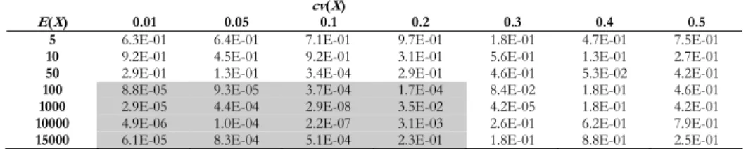
Table 1 shows the p-values of the Shapiro-Wilk normality test computed on the observed values of the sample mean Ye.
TABLE 1
p-values of the S-W normality test computed on the sample means
cv(X)
E(X) 0.01 0.05 0.1 0.2 0.3 0.4 0.5
5 6.3E-01 6.4E-01 7.1E-01 9.7E-01 1.8E-01 4.7E-01 7.5E-01
10 9.2E-01 4.5E-01 9.2E-01 3.1E-01 5.6E-01 1.3E-01 2.7E-01
50 2.9E-01 1.3E-01 3.4E-04 2.9E-01 4.6E-01 5.3E-02 4.2E-01
100 8.8E-05 9.3E-05 3.7E-04 1.7E-04 8.4E-02 1.8E-01 4.6E-01
1000 2.9E-05 4.4E-04 2.9E-08 3.5E-02 4.2E-05 1.8E-01 4.2E-01
10000 4.9E-06 1.0E-04 2.2E-07 3.1E-03 2.6E-01 6.2E-01 7.9E-01
15000 6.1E-05 8.3E-04 5.1E-04 2.3E-01 1.8E-01 8.8E-01 2.5E-01
Non-normality appears evident when E(X)100 and cv(X)0.2 (the shaded part of Table 1). In order to appreciate the effects of error model (2) on the con-trol chart, we have focused on the in-concon-trol and out-of-concon-trol situations.
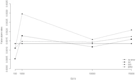
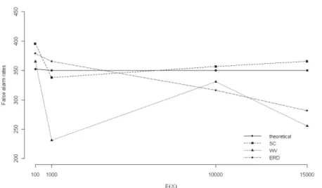
In order to study the effects of error model (3) on the false alarm rates, the in-control conditions were simulated for E(X)100 and cv(X)0.2 of the unobserv-able X. With fixed sample size n=5, we generated 108 samples for each condition.
Results are summarized in Figure 1 where the continuous line, denoted as “no errors”, corresponds to 0.00135, i.e. the probability, for the undisturbed process and in the error-free case, of a signal below the LCL (or above the UCL). Con-tinuous lines are used for the false alarm rates above the UCL and dotted lines are used for the false alarm rates below the LCL.
Figure 1 – False alarm rates from 108 replications (dotted lines for the values below the LCL,
Figure 1 shows a marked asymmetric behaviour: false alarm rates below the
LCL are lower than the false alarm rate in the error-free case (0.00135), while the false alarm rates above the UCL are systematically greater than this value.
When considering the out-of-control situation, a shift in the mean of the non-observable X, from to 1, corresponds to a standardized shift of magnitude
1
(9)
In the presence of shift (9) in X, the expected value of the response Ye is
2
1
( e)
E Y e (10)
and the corresponding standardized shift in the monitored Ye is
2 2 2 2 2 1 0 1/2 2 2
2 2 2
1 ( 1) ( 1)
e e Y Y m p p e e e e e (11)
For non-zero and m, the denominator in (11) is greater than 1, and there-fore Ye . As a result, measurement errors lead to a smaller shift in the
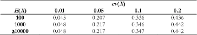
ob-served response Ye, which means that the change is more difficult to detect. Ta-ble 2 shows the values of Ye corresponding to a shift 0.5 for those values of E(X) and cv(X) in question, where the reduction in the shift is evident for small values of E(X) and cv(X).
TABLE 2
Values of Ye corresponding to a standardized shift of magnitude ||=0.5
cv(X)
E(X) 0.01 0.05 0.1 0.2
100 0.045 0.207 0.336 0.436
1000 0.048 0.217 0.346 0.442
10000 0.048 0.217 0.347 0.442
One of the most commonly-used measures for evaluating the statistical prop-erties of control charts is the ARL (Average Run Length). For the Ye-chart, the theoretical ARL for shifts of magnitude e
1
( Ye) ( ( 3 Ye ) ( 3 Ye ))
ARL n n (12)
The ARL values corresponding to the Ye in Table 2 are reported in Table 3
TABLE 3
Theoretical values of ARL for the Ye in Table 2
cv(X)
E(X) 0.01 0.05 0.1 0.2
100 352.49 170.99 81.13 46.50
1000 350.34 161.06 76.27 45.09
10000 350.31 160.96 76.23 45.07
Expression (12) is based on the normality assumption of the sample statistic used in the chart, although we noticed that measurement errors lead to departures from the Normal distribution. Thus, in order to assess the effects of the two-component measurement error, we conducted a simulation study of the out-of-control situations. For each combination of cv(X) and E(X) in Table 1, we fixed shifts of magnitude 0.5 in the variable X, and estimated the off-target ARLs
of the Ye-control-charts. Each condition was again replicated 108 times: results for negative and positive shifts are summarized in Table 4.
TABLE 4
Estimated ARLs (= -0.5 left values and = +0.5 right values within each parenthesis)
cv(X)
E(X) 0.01 0.05 0.1 0.2
100 (380.5 282.7) (265.4 116.6) (121.2 57.8) (59.3 37.0)
1000 (392.3 279.9) (279.2 108.1) (117.2 54.6) (57.5 36.1)
10000 (368.9 289.0) (271.7 106.8) (118.0 54.3) (58.0 35.9)
15000 (384.8 271.0) (269.8 104.9) (118.3 53.7) (57.0 36.1)
Table 4 confirms the asymmetric effect of measurement errors. The ARLs for positive shifts are smaller than the corresponding ARLs for negative shifts. As one would have expected, the values shown in the table tend to differ from the theoretical ARL values shown in Table 3, in particular as E(X) increases.
4. THE DESIGN OF THE CONTROL CHARTS UNDER THE TWO-COMPONENT ERROR MODEL
The results obtained so far show that error-model (3) leads to important modi-fications in the performances of the Shewhart control chart, which in turn result in problems in the practical use of such monitoring algorithms. In particular, we noticed departure from normality, a marked asymmetric behaviour, and a general difficulty in assessing the performances of the control chart itself.
When the distribution of the observable quality characteristic is known, exact methods can be used for analytically computing the control limits for the desired Type I risk. In our model (3) the observable quality characteristic Ye is modelled as the sum of a normal variable, Ye, and the product of a normal variable, X, by a log-normal variable e. The analytical derivation of this distribution is not im-mediate. Tools for computing the product of random variables have been pro-posed, for instance by Roahtgi (1976) and Springer (1979), the last mostly relying on Mellin transforms. The analytic derivation, and the further implementation and computation of these results, are, when possible, rather complicated, as Glen
et al. (2004) pointed out. Moreover, once obtained the distribution of the product, say Yp, the further difficulty of obtaining the distribution Ye as the convolution of Yp and has to be faced.
In general, the charts constructed by the exact method are not in a form famil-iar to practitioners and quality engineers who are used to conventional X charts (Bai and Choi, 1995, Chan and Cui, 2003). Therefore, other approaches will be examined.
4.1 The weighted variance method
For skewed distributions Choobineh and Ballard (1987) suggest a weighted vari-ance (WV) method based on the semivarivari-ance approximation of Choobineh and Branting (1986). Following this mainstream, Bai and Choi (1995) propose an inter-esting heuristic WV method without distributional assumptions, which will be syn-thetically illustrated. This method provides asymmetric control limits that keep into account the direction and degree of skewness, that is estimated by using different variances in computing upper and lower control limits for skewed populations.
The WV method, like the Shewhart method, uses the standard deviation for setting the control limits. However, it differs from the Shewhart method since the standard deviation is multiplied by two different factors. One factor is used for the UCL, while the other is used for the LCL. Let PX be the probability that the random variable X is less or equal to its mean X. Then the UCL factor is 2PX , and the LCL factor is 2(1PX). The control limits of the X chart based on the WV method are
3 2
3 2(1 2 )
X
X X
X
X X
UCL P
n
LCL P
n
(13)
For using in practice the control chart (13) based on the WV method, both PX and the process parameters must be estimated. Let X Xi1, i2,...,Xin, i=1,2,...,r, be
distribution and parameters are unknown Bai and Choi (1995) propose the WV
X Chart:
' 2
' 2
ˆ
3 2(1 )
ˆ
3 2
WV X L
WV
WV X U
R
LCL X P X W R
d n
CL X
R
UCL X P X W R
d n
(14)
where X (1 ( ))nr
ri1 nj1Xij , (1 ) 1r i i
R r
R , and Ri is the range of thei-th subgroup that is used to estimate the standard deviation. Further, the weight ˆ
X
P estimates the probability that the random variable X is less than or equal the mean ( )E X :
1 1 ( ) ˆ r n ij i j X X X P nr
(15)with ( ) 1 x for x0 and ( ) 0 x for x < 0. The values of d2 that appear in (14), for given n and PX, can be computed using the method described by Bai and Choi (1995) whereas constants WL 3 2(1PX) d2 n and
2
3 2
U X
W P d n for selected combinations of n and PX are listed in Table 1 of Bai and Choi (1995).
The practical use of the WV method, with respect to the Shewhart method, doesn’t imply an increase of the computational complexity since it requires only the estimation of the probability PX from the preliminary r samples from the in-control process (i.e. Phase I data).
4.2 The skewness correction method
Also the skewness correction (SC) method (Chan and Cui, 2003 and Yazici and Kan, 2009)) correct the conventional Shewhart chart according to the skewness of the distribution. This approach is based on the Cornish-Fisher expansion reported by Johnson and Kotz (1970). For the standardized random variable X with mean 0, standard deviation 1 and skewness k3, the LCL, CL and UCL of a standardized
control chart for individual observation based on the SC method are:
4 3 3 2 3 3 1 0.2 k LCL k
,CL0,
For the general case of subgroups of size n and unknown parameters, Chan and Cui (2003) propose the SC X Chart:
* 3 * 2 2 3 * 3 * 2 2 3 ˆ
4 (3 )
3 ˆ
1 0.2
ˆ
4 (3 )
3 ˆ
1 0.2
SC L
SC
SC U
k n R
LCL X X A R
d n
k n
CL X
k n R
LCL X X A R
d n k n (16)
where kˆ3 is the estimated sample skewness
3
3 2
1 1 1
1 1 1
1 ˆ
3 ( )
r n
ij
r n i j
ij nr i j
X X
k
nr X X
(17)Constants *
L
A and *
U
A are listed in Table 1 of Chan and Cui (2003). The SC method consists in a semi-parametric approach that requires the first three mo-ments of the distribution, even if the distributional form has not to be explicited. Compared with the Shewhart approach, the SC method needs the estimation of the skewness parameter k3 which represents only a negligible increase in the
complexity of the method.
4.3 The empirical reference distribution method
Chakraborti et al. (2001) presented an extensive overview of the literature on univariate distribution-free control charts, and subsequent scientific works, among which we quote Vermaat et al. (2003), Chakraborti et al. (2004) and by Chakraborti and Van de Wiel (2008), have confirmed the growing interest in this issue.
One of the distribution-free control charts discussed in Chakraborti et al. (2001) was previously proposed by Willemain and Runger (1996). This proposal makes it possible to design both one-sided and two-sided control charts from a sufficiently large in-control (or, a reference) sample, by selecting the control limits as specific order statistics of the variables to be charted. As stated by the authors the availabil-ity of a large preliminary data set from the undisturbed process (in-control) is a nec-essary condition for the nonparametric design of control charts, since estimation of extremes percentiles corresponding to a large on-target average run length (ARL) would be impossible without a large number of observations.
sam-ples. Here Z is Ye E Y( e) and the zi values are the observed sample means yie. We assume that m preliminary samples are taken from the undisturbed process.
Let z(k) be the k-th order statistic in the sample, k=1, 2, ..., m, (for basic order
statistics theory, see for example David and Nagaraja, 2004), and z(m) be the
larg-est value of the z(k). By convention z 0 and zm1 . The m order
statis-tics divide the theoretical range of Z into m+1 equally probable intervals.
If the control limits are defined as LCLERDz k and UCLERD z s , with 0 k s m, then
Pr[ k s ]
P z Z z (18)
is the probability that a value of the sample statistic Z falls within the control lim-its LCLERD and UCLERD.
Probability P has a Beta distribution that depends only on m and on the num-ber b=s-k of intervals within the control limits
( , 1)
P Beta b m b (19)
Assuming the independence of the plotted points, the number R of plotted points between alarms has a geometric distribution with parameter 1P. For a given P, the in-control ARL is
1
( | ) (1 )
ARL E R P P (20)
Since the z(k) are the observed values generated by the random variables Z k ,
the ARL itself is a random variable with Inverted–Beta distribution
1 1
!
( ) ( 1)
( 1)!( )!
h m
m
h ARL ARL ARL
b m b
(21)
with expected value
( ) m
E ARL
m b
(22)
and standard deviation
1/2 2
. .( )
( ) ( 1 )
bm s d ARL
m b m b
(23)
It is also possible to compute the quantiles of the ARL distribution using the relationship
Pr[ARL A] Pr[ P 1 1/ ]A (24)
The ERD method allows also to assess the performances of the control chart in the out-of control-situations by evaluating the expected ARL using a shift pro-cedure. Details are summarised in the Appendix.
5. COMPARISONS OF THE DIFFERENT METHODS
We compare the performances of the three methods when the measurement error model (3) is considered in designing control charts for the mean level of the observable quality characteristic Ye. We select the situation where cv(X)=0.01 among the cases examined in Section 3 (the other cases can be treated similarly).
To build WV and SC control charts we simulate a preliminary data set of r=50 independent and “in-control” subgroups of size n=5 for the E(X) values of inter-est. The sample estimates are reported in Table 5.
Constants WL, WU *
L
A , and *
U
A obtained by interpolating the values of Table 1 in Bai and Choi (1995) and Table 1 in Chan and Cui (2003) respectively, are re-ported in Table 6, together with the control limits of the WV and SC control charts.
TABLE 5
Sample estimates from r=50 simulated samples for cv(X)=0.01 E(X)
100 1000 10000 15000
e
Y 164.918 1534.168 15432.606 22910.358
e
Y
R 40.970 373.927 3688.634 5648.898 ˆe
Y
P 0.524 0.492 0.492 0.528
3
ˆ
k 0.441 0.284 0.161 0.194
For building ERD based control charts with performances comparable with the 3 limits charts just obtained, we choose m=10000 and b=9973, thus from equation (22) we have (E ARL) 370.4
In order to obtain a reasonable chart performance, we set k=14 and conse-quently LCLERD z 14 and UCLERDz9987, leaving 14 blocks below the LCL
and 14 blocks above the UCL, allowing, in this way, a well-behaving ARL. We created the undisturbed preliminary data set by generating the m samples of size n=5 from the observable response Ye. After obtaining the sample means
e i
TABLE 6
WV and SC constants and WV, SC and ERD control limits for cv(X)=0.01
E(X)
100 1000 10000 15000
L
W 0.518 0.580 0.580 0.516
L
W 0.590 0.580 0.580 0.590
* U
A 0.635 0.615 0.600 0.604
* L
A 0.527 0.545 0.560 0.556
WV
LCL 143.696 1317.141 13291.723 19995.527
WV
UCL 189.099 1750.896 17570.538 26245.467
SC
LCL 143.331 1330.563 13367.369 19770.695
SC
UCL 190.940 1764.317 17646.184 26323.416
ERD
LCL 143.341 1336.275 13363.672 20027.123
ERD
UCL 189.062 1768.048 17589.563 26305.440
5.1. Comparison of the in-control performances
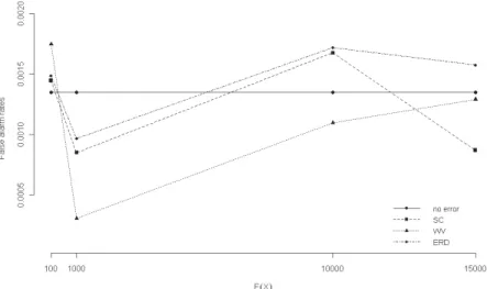
The in-control performances of the charts with the control limits reported in Table 6, are assessed by generating 108 samples (n=5) from the in-control
proc-ess, for every combination of E(X) and cv(X)=0.01. The observed false alarm rates, due to a signal above the upper control limits and below the lower control limits, are shown in Figures 2 and 3 respectively. In both figures, the “no-error” value equal to 0.00135 is denoted as a continuous line.
Figure 3 – False alarm rates below the LCLs.
Charts behaviour, when compared with Figure 1, shows a strong improve-ment: the false alarm rates now follow a random pattern around the theoretical value 0.00135, without evidence of asymmetry. Moreover, the false alarm rates of the SC and ERD charts are closer to the no-error value than the WV charts which show a less stable behaviour to the changes of E(X).
5.2. Comparison of the out-of-control performances
For each value of E(X), when cv(X)=0.01, we fixed shifts of magnitude 0.5
in the variable X. The off-target ARLs were estimated by performing 108 replications of the experiment. Results are reported in Figures 4 and 5.
Figure 5 – Estimated ARLs=+0.5.
In these figures the benchmark “theoretical” lines, corresponding to the values computed using formula (12) and appearing in Table 3 (first column), are re-ported. The estimated out-of-control ARLs do not show a systematic asymmetric behaviour, SC and ERD show comparable ARLs that seem to have more steady performances than the WV control charts.
As a conclusion, when the data are contaminated by the proposed two-component error model, the SC and ERD based X -control charts show similar performances being less sensitive to the presence of measurement errors.
6. CONCLUDING REMARKS
Studies of the effects of measurement errors on monitoring algorithms tradi-tionally use the Gaussian additive error model. However, it has often been pointed out that, in connection with particular measurement devices, a more real-istic error model ought to be considered.
In this paper we have proposed an extension of the usual error model (1) to cover a more general situation, by introducing the structure of the two-component error model (2). The two-two-component error model was proposed for uncertainty measurement in analytical chemistry and environmental monitoring. Model (2) jointly considers a constant error-component, which reveals its effects at low measurement levels, and a proportional error-component, which becomes significant at higher levels of measurement. The overall picture of measurement uncertainty given by the two-component error model is very realistic and re-sponds to several among the improving requirements from the literature and the practice of statistical process control.
knowledge have up until now been proposed separately. We have stressed the point that the proposed error model can lead to a significant departure from the normal distribution, and have an important impact on control chart performance. This happens because, while the additive error basically inflates the variance of the observable response Ye, the proportional error component leads to a re-markable asymmetry in the performance of the mean control chart.
Results indicate that when the process is in-control, the false alarm rate above the UCL is greater than the theoretical false alarm probability, while the false alarm rate below the LCL is smaller. This is an important issue, since false alarms may cause a series of expensive, unnecessary actions or regulations. Moreover, asymmetry can complicate monitoring management. The effects of the two-component error model are also evident in the out-of-control situation: the ARL
for negative shifts is always greater than the corresponding ARL for positive shifts.
In order to take errors into account when designing the control chart, we have compared by simulation the use of several control chart design methods. Our re-sults indicate that the SC and ERD methods of constructing X control chart improve the chart performance when the process is in-control, in the sense that the observed false alarm rates are symmetric and in agreement with theoretical false alarm probability. Also for the out-of-control cases performance of the SC and ERD charts do not show an asymmetric behaviour. As a conclusion we state that SC and ERD based X -control charts are less sensitive to the presence of measurement errors.
However, the large number of observations from the so-called Phase I, neces-sary to ascertain the control limits in the ERD method, may be a potential limita-tion in practice. Therefore the solulimita-tion based on the skewness correclimita-tion (SC) method might appear the best choice at the price of assuming the existence of the first three moments of the distribution. In this case the design of the control chart is based on the estimation of the first three moments of the distribution.
Department of Statistics DANIELA COCCHI
APPENDIX
A.1 ARL COMPUTATION FOR THE ERD METHOD IN THE OUT-OF CONTROL CASE
For the out-of-control situation, given the chosen control limits, the corre-sponding expected off-target ARL can be evaluated using a shift procedure. It is based on the idea that a shift in the process level will modify the number of ob-served order statistics falling within the control limits. Thus, the problem of as-sessing off-target ARL is transformed into the assessment of on-target ARL with a smaller number of intervals within the control limits.
In the two-sided chart, we have LCLERD z k and UCLERD zk b . If an assignable cause leads to an upward shift in the mean, then all order statistics will shift upwards in a way such that zk b k ' takes the position formerly held by
k b
z . The shift decreases the number of intervals below the UCLERD, from b+k
to b+k-k’, while it increases the number of intervals above the LCLERD. How-ever, as Willemain and Runger (1996) pointed out, this interval-shifting is not symmetric since the decrease in the number of intervals in the upper part of the in-control region is only partially compensated by the increase in the number of intervals on the lower part by some fractional amount.
Thus, for a given upward shift, b’=b+k-fk’ intervals (0<f<1) remain, where k’
is the decrease in the number of intervals within the control limits. If the ob-served spacings between the order statistics are used as values of the shifts, it is possible to estimate the off-target E(ARL) at those particular values of shift, and thus the value k’ is an integer.
A downward shift can be treated similarly: a negative shift reduces the number of intervals at the low end of the in-control region, and is partially compensated by an increase in the number of intervals on the high end by some fractional amount.
The effectiveness of the aforesaid method of evaluating the expected off-target
ARL depends on the specification of a value for the fractional amount f. The choice of f may be critical, in the sense that a modification in the E(ARL) values for a given shift may be sensitive to this choice. Since there is no general criterion for a satisfactory choice of f, we conducted a preliminary set of simulations using several values of f. We found that small values of f lead to unreasonable and un-stable results while large values of f give better results. Thus we decided to set the
f value at 7/8.
Let us first consider the case of an upward shift. We denote with z j the j-th order statistics, and thus
1 UCLERD z j
(A1)
Since in our case the z j values correspond to the ordered values of yej, the estimated standard deviation of the sample means e
j
y (j=1,2,...,m) is
1/2 2 1
ˆ ( )
1 e m j Y i z z m
(A2)where 1 1
m
j j
z m z
.Therefore, the empirically estimated standardized shift in Ye is
1 ˆ ˆ e e Y Y
(A3)
which corresponds to an upward shift that moves a z j into the position of
UCLERD, while the empirically estimated standardized shift in Ye, corresponding to a shift of size ˆYe in Ye, is
ˆ ˆ e
e Y
Y n
(A4)
We have to look for those values of ˆYe that provide the best approximation of the values of Ye and estimate the off-target E(ARL) at those particular values of shift.
Table A1 shows an extended version of the results for E(X)=100 and
cv(X)=0.01. A summary of the results in all the other cases is given in Table A2. In Table A1 the column labelled as “ j ” shows the positions of the ordered sam-ple means z j . Column “1” contains the values of the observed spacings be-tween the UCLERD and the order statistic z j , according to equation (A1), while the next two columns show the values of ˆ e
Y
and ˆ e Y
computed according to (A3) and (A4) respectively. For each value of 1 (ˆYe), we computed the number of intervals within the control limits b’=b+k-fk’, as described above. The values of E(ARL) and s.d.(ARL) conditional on shift 1 (ˆYe) are calculated by equa-tions (22) and (23) respectively, with b’ in the place of b, i.e.:
( ) ( ')
E ARL m m b and s d ARL. .( ) ( ' b m m b(( ') (2 m 1 b')))1/2. The
col-umns “2.5%” and “97.5%” show the percentiles of the distribution of the ARL
For E(X)=100 and cv(X)=0.01 the standardized shift in Ye is 0.045 e
Y
(Table 2), which is best approximated by ˆ e 0.052 Y
, with a corresponding
E(ARL)=337.6.
For a downward shift 1LCL z j , ˆYe and ˆYe are defined according to the usual equations (A3) and (A4). In this case, the best approximation to Ye is obtained by ˆYe 0.044 with a corresponding E(ARL)=327.9.
TABLE A1
Off-target ARL computations for E(X)=100 and cv(X)=0.01 (ˆYe 7.51).
j z j 1 ˆYe ˆYe b+k-k’ b+k-fk’ E(ARL) s.d.(ARL) 2.5% 97.5%
Upward shift
9987 UCLERD=189.062 0.000 0.000 0.000 9973 9973.000 370.4 3.7 254.7 537.2
9986 188.887 0.175 0.023 0.010 9972 9972.125 358.7 3.5 248.2 517.4 9985 188.887 0.175 0.023 0.010 9971 9971.250 347.8 3.5 242.0 498.9 9984 188.186 0.876 0.117 0.052 9970 9970.375 337.6 3.4 236.1 481.6
Down ward shift
19 144.380 -1.038 -0.139 -0.062 9968 9968.625 318.7 3.2 225.2 450.3 18 144.078 -0.737 -0.098 -0.044 9969 9969.500 327.9 3.3 230.5 465.4
17 143.870 -0.528 -0.070 -0.032 9970 9970.375 337.6 3.4 236.1 481.6 16 143.784 -0.443 -0.059 -0.026 9971 9971.250 347.8 3.5 242.0 498.9 15 143.516 -0.175 -0.023 -0.010 9972 9972.125 358.7 3.6 248.2 517.4
14 LCLERD=143.341 0.000 0.000 0.000 9973 9973 370.4 3.7 254.7 537.2
TABLE A2
Off-target ARL computations for cv(X)=0.01
j z j ˆYe b+k-k’ b+k-fk’ E(ARL) s.d.(ARL) 2.5% 97.5%
( ) 1000
E X ˆYe71.13
upward shift 9982 1760.645 0.044 9969 9968.5 327.9 3.3 230.5 465.4 downward shift 20 1343.494 -0.045 9967 9967.75 310.1 3.3 220.1 436.0
( ) 10000
E X ˆYe698.52
upward shift 9982 17503.48 0.055 9968 9968.625 318.7 3.2 225.2 450.3 downward shift 19 13435.53 -0.046 9968 9968.625 318.7 3.2 225.2 450.3
( ) 15000
E X ˆYe1063.46
upward shift 9980 26192.59 0.047 9966 9966.875 301.9 3.0 215.2 422.6 downward shift 23 20152.75 -0.053 9964 9965.125 286.7 2.9 206.2 398.1
ACKNOWLEDGEMENTS
REFERENCES
D.S. BAI, I.S. CHOI, (1995), X and R control charts for skewed populations, “Journal of Quality Technology”, 27, pp. 120-131.
R.K. BURDICK, C.M. BORROR, D.C. MONTGOMERY, (2003), A review of methods for measurements
sys-tems capability analysis. “Journal of Quality Technology”, 35, pp. 342-354.
R. CAULCUTT, R. BODDY, (1983), Statistics for Analytical Chemists, Chapman and Hall, London. S. CHAKRABORTI, P. VAN DER LAAN, S.T. BAKIR, (2001), Nonparametric control charts: an overview and
some results, “Journal of Quality Technology” 33, pp. 304-315.
S. CHAKRABORTI, P. VAN DER LAAN, M.A. VAN DEWIEL, (2004), A class of distribution-free control
charts, “Applied Statistics”, 53, pp. 443-462.
S. CHAKRABORTI, P. VAN DER LAAN, M.A. VAN DEWIEL, (2008), A nonparametric control chart based
on the Mann-Whitney statistic, in N. Balakrishnan, E.A. Peña, M.J. Silvapulle, M.J. (eds.), “Beyond parametrics in interdisciplinary research: Festschrift in honour of professor Pranab K. Sen”, Institute of Mathematical Statistics Collections, Beachwood USA, Vol. 1, pp. 156-172.
L.K. CHAN, H.J. CUI, (2003), Skewness correction X and R charts for skewed distributions, “Naval Research Logistics”, 50, pp. 555-573.
F. CHOOBINEH, J.L. BALLARD, (1987), Control-limits of QC charts for skewed distribution using
weighted variance, “IEEE Transactions on Reliability”, 36, pp. 473-477.
F. CHOOBINEH, D. BRANTING, (1986), A simple approximation for semivariance, “European Jour-nal of OperatioJour-nal Research”, 27, pp. 364-370.
D. COCCHI, M. SCAGLIARINI,(2010), A robust approach for assessing misclassification rates under the
two-component measurement error model, “Applied Stochastic Model in Business and Indus-try”, 26, pp. 389-400.
H. DAVID, H. NAGARAJA,(2003), Order Statistics 3-rd ed., John Wiley & Sons, London.
R.D. GIBBONS, D.E. COLEMAN, R.F. MADDALONE, (1997), An alternative minimum level definition for
analytical quantification, “Environmental Science and Technology” 31, pp. 2071-2077. A.G. GLEN, L.M. LEEMIS, J.H DREW, (2004), Computing the distribution of the product of two continuous
random variables, “Computational Statistics & Data Analysis” 44, pp. 451-464. N.L. JOHNSON, S. KOTZ, (1970), Continuous Univariate Distributions-1, Wiley, New York. G. JONES,(2004), Markov chain Monte Carlo estimation for the two-component model,
“Technomet-rics”, 46, pp. 99-107.
T. KANAZUKA,(1986), The effects of measurement error on the power of X-R charts, “Journal of Quality Technology”, 18 pp. 91-95.
K.W. LINNA, W.H. WOODALL,(2001), Effect of measurement error on Shewhart control charts, “Journal of Quality Technology”, 33, pp. 213-222.
K.W. LINNA, W.H. WOODALL, K.L BUSBY,(2001), The performances of multivariate effect control charts in
presence of measurement error, “Journal of Quality Technology” 33, pp. 349-355.
P.E. MARAVELAKIS, (2007), The effect of measurement error on the performance of the CUSUM control chart, Proceedings of the 2007 IEE IEEM, pp. 1399-1402, Singapore. P.E. MARAVELAKIS, J. PANARETOS, S. PSARAKIS,(2004), EWMA chart and measurement error,
“Jour-nal of Applied Statistics”, 31, pp. 445-455.
D.L. MASSART, B.G.M. VANDINGSTE, S.N. DEMING, Y. MICHOTTE, L. KAUFMAN,(1988), Chemometrics; a
Textbook, Elsevier, Amsterdam.
H.J. MITTAG, D. STEMANN,(1998), Gauge imprecision effect on the performance of the X S control
chart, “Journal of Applied Statistics”, 25, pp. 307-317.
D.C. MONTGOMERY, G.C RUNGER,(1993), Gauge capability and designed experiments. Part I: basic
D.M. ROCKE, B. DURBIN, (2001), A model for measurement error for gene expression arrays, “Journal of Computational Biology”, 8, pp. 557-569.
D.M. ROCKE, S. LORENZATO, (1995), A two-component model for measurement error in analytical
chem-istry, “Technometrics”, 37, pp. 176-184.
D.M. ROCKE, B. DURBIN, M. WILSON, H.D. KAHN, (2003), Modeling uncertainty in the measurement of
low-level analytes in environmental analysis, “Ecotoxicology and Environmental Safety”, 56, pp. 78-92.
V.K. ROHATGI, (1976), An Introduction to Probability Theory Mathematical Statistics, John Wiley & Sons, New York.
M.D. SPRINGER, (1979), The Algebra of Random Variables, John Wiley & Sons, New York. M.B. VERMAAT, R.A. ION, R.J.M.M. DOES, C.A.J. KLASSEEN, (2003), A comparison of Shewhart
individu-als control charts based on normal, non-parametric, and extreme-value theory, “Quality and Reli-ability Engineering International” 19, pp. 337-353.
T.R. WILLEMAIN, G.C. RUNGER, (1996), Designing control charts using an empirical reference
distribu-tion, “Journal of Quality Technology”, 28, pp. 31-38.
A. WILSON, M. HAMADA, M. XU, (2004a), Assessing Production Quality with Nonstandard
Measure-ment Errors, “Journal of Quality Technology”, 36, pp. 193-206.
M.D. WILSON, D.M. ROCKE, B. DURBIN, H.D. KAHN, (2004b), Detection limits and goodness-of-fit
meas-ures for the two-component model of chemical analytical error, “Analytica Chimica Acta”, 509, pp. 197-208.
B. YAZICI, B. KAN (2009), Asymmetric control limits for small samples, “Quality & Quantity”, 43, pp. 865-874.
SUMMARY
Effects of the two-component measurement error model on X control charts