Thesis

(1)

(2)

I would like to thank several individuals for their help with this project. First of all, I would like to thank Dr. Virginia Gray. Without her help as my advisor, this project would not have been possible. She has served as my mentor, advisor, and favorite professor at UNC ever since I met her during my freshman year. Her guidance has led me on my current path to

graduate school, and I cannot thank her enough for all of her help. She is a fantastic person, and was immensely helpful as my advisor. Next, I want to thank the two other members of my thesis committee, Dr. Frank Baumgartner and Dr. Thomas Carsey. Their insight helped me make some key revisions that improved my thesis. I also want to thank Dr. Stephen Gent, who guided all of the thesis writers through the general process. His help was invaluable.

(3)

I. Introduction

For the past few years, the Patient Protection and Affordable Care Act (ACA) has been a

constant source of debate among the American public. Whether it has been in the halls of

Congress or on the street corners of U.S. cities, everyone seems to have an opinion on this

divisive law. Many scholars agree that “Obamacare,” as it is known colloquially, is an integral

part of the rise in ideological polarization among our lawmakers. Due to this political

polarization, implementation of the Affordable Care Act has varied across the United States.

Generally, states with liberal legislatures have embraced the act, while states with conservative

legislatures have attempted to block it (Obama Care Facts 2013, 1). This ideological divide has

very important implications for citizens. Many of the provisions of the law contain health

insurance provisions that will affect the daily lives of nearly every citizen. The implementation

of these provisions is essential to their success. My thesis seeks to discover the true effects of the

ideological divide on the Affordable Care Act by doing a state-by-state analysis. In doing this, I

answer the question: “How have state government actions altered the effectiveness of the

Affordable Care Act?”

I answer this question because of its importance in current American politics. Because it

deeply affects the lives of citizens, it is the duty of researchers like myself to investigate the

ACA thoroughly. This thesis provides a guide with which to examine future state

implementation actions. In a broader sense, this study is also important because it examines the

manner in which truly federal policies work. When I mention the term “truly federal”, I mean

that the ACA requires both the national and state governments to cooperate on implementation.

While the ACA is a national law, states were given a considerable amount of power in its

(5)

governments in implementing federal laws. Because of its current relevance and its broader

implications for federal policies, I study ACA implementation.

The next section of this study presents a review of current literature on the Affordable

Care Act. By summarizing this literature, I provide a scholastic introduction to the Affordable

Care Act for the reader. After providing a summary of this literature, I describe how my thesis

fits into the existing research and expands upon it. Next, I provide a theoretical argument for the

topic, outlining the manner in which state government actions impact Affordable Care Act

implementation. In doing this, I present a causal mechanism, which describes each phase of this

process in detail. The causal mechanism leads to my hypothesis, which predicts a link between

state government actions and effectiveness of the ACA. I then propose to test the hypothesis by

testing the impact of state government actions on two goals of the Affordable Care Act: “better

access to care” and “more affordable coverage”. Next, I present several regression analyses to

test these goals. For goal one, while exchange implementation had some effect, states that

expanded Medicaid were most likely to provide “better access to care” for citizens (goal one).

The result for goal two is less conclusive. While there is some evidence to support the hypothesis

that state government actions impacted the goal of “more affordable coverage”, there were

conflicting results among my models. Ultimately, I conclude that states that acted on exchange

implementation or expansion of Medicaid are more likely to have positive results than those that

(6)

II. Literature Review

Pre-First Enrollment Period

The existing literature on the Affordable Care Act covers a broad range of topics and

theirrelationship with the law. As discussed in this review, the current research focuses on

individual states and their specific outcomes. It also discusses individual health issues and their

relation to the Affordable Care Act. However, while there is a large amount of research on

specific states and issues, the current literature lacks a comprehensive analysis that describes the

link between state government actions and effectiveness for all 50 states. As I detail later, this is

where my research will fit in. By providing a causal mechanism to describe ACA outcomes for

all 50 states, I add to the current research base on the topic.

One of the major works that addresses implementation of the ACA is by Haeder and

Weimer (2013). Their article provides two methods to analyze state government actions toward

implementation of the law: whether a state joined a lawsuit against the ACA, and whether a state

created its own insurance exchange. According to this research, 22 states joined a lawsuit, while

28 did not. As for creating their own exchanges, 15 initially created one, while 35 did not. It is

important to note that these statistics slightly changed as the law’s implementation moved

forward. These statistics present a general trend among the states. In states that are under

Democratic control (specifically of the legislature), there is much less opposition toward the

ACA. Conversely, states that are controlled by Republicans tended to take negative action

toward the ACA’s implementation. These metrics, as well as the context behind them, are vital in

analyzing state government actions toward the law.

The authors also describe several different themes of exchange implementation. Divided

(7)

Democrat-leaning states moved quickly after enactment of the ACA and established exchanges between

December 2010 and July 2011” (Haeder and Weimer 2013, 38). The other end features

“Republicans outside Washington, D.C. [that] found themselves confronted with an interesting

dilemma: either support the implementation of the ACA and develop local, conservative

solutions or come out vocally against it and refuse to cooperate at all costs” (Haeder and Weimer

2013, 38). It is extremely important to consider each state’s individual dilemmas when analyzing

implementation of the Affordable Care Act. Once again, this article illustrates the general trend

in state government actions on the ACA among party lines. While the metrics at the beginning of

the paper provide important data on the nation as a whole, it also includes some specific cases

that provide important context.

While Haeder and Weimer (2013) briefly mention these important specific cases,

Benjamin, Slagle, and Jones (2013) expand on them. This article, which mentions the Haeder

and Weimer paper as a starting point, provides an in-depth view of states like “Oregon, [in

which] the adoption of a rigorous rate review process resulted in […] lowered premium rates”

(Benjamin, Slagle, and Jones 2013, 48). It also discusses “New York, [which had] a radical

reduction in premiums (in some cases by nearly 50 percent) and the launch of an

all-payer-claims database that is expected to further reduce costs and regularize the health care

marketplace” (Benjamin, Slagle, and Jones 2013, 48). Examples like these provide an excellent

idea of the success that the law has had in states that took positive actions towards implementing

it. While this article presents cases of successful implementation, it lacks examples of states that

did not take positive actions on the law. A more complete analysis of ACA implementation

(8)

Along with these specific state cases, Benjamin, Slagle, and Jones (2013) also address

national measures that were adopted to ease state implementation as a whole, especially in states

that did not accept the ACA right away. One such measure that they address is “postponing the

employer mandate [until 2015, which] will potentially beneﬁt the state-based individual

insurance exchanges by increasing the number of covered lives in those exchanges” (Benjamin,

Slagle, and Jones 2013, 38). The inclusion of this national policy reveals an important trend

about ACA implementation. Because many states were vehemently opposed to implementing the

law from the outset, the national government had to adjust its policies. This article, combined

with Haeder and Weimer’s (2013) analysis, provides excellent detail about implementation of

the ACA as well as each state’s actions toward it.

While the Benjamin article presents a broadened view of health care effectiveness by

focusing on the system as a whole, Martin, Strach, and Schackman (2013) focus on a single

issue. In narrowing its view to just HIV care, this article provides another way to evaluate the

effectiveness of the ACA. The article does this by discussing the link between state government

action and success. The authors found that, “States such as California and Maryland that have

strong political commitment to implement the ACA (including Medicaid expansion) […] are

likely to do better than under current conditions” (Martin, Strach, and Schackman 2013, 95). By

accounting for states’ actions toward the ACA in the context of HIV care, the authors were able

to find a positive link between state government actions and effectiveness. Later in the paper, the

authors address states that did not take action on the ACA. According to their findings, “there

may be no change or possibly worse HIV health outcomes in states without political commitment

(9)

link between state government actions and effectiveness of the ACA. However, a more complete

analysis would feature many different health outcomes, not just a single issue.

Post-First Enrollment Period

While there is a plethora of articles on the time before the first enrollment period, the

research from after the first enrollment period is much more limited. However, despite these

limitations, there are some key studies on this period. One of the major analyses on this period is

by Blumenthal and Collins (2014). This study provides a report on the progress of the Affordable

Care Act nationwide. In completing this report, Blumenthal and Collins (2014) come to three

main conclusions. First, they conclude that, “As the number of individuals benefitting from the

law grows, its wholesale repeal will grow less likely, although the law could still be importantly

modified in the future” (Blumenthal and Collins 2014, 281). This consideration is important

when examining the implementation of the law. If the law were to be repealed in the future,

current analyses would be rendered mostly irrelevant. However, because the law will not be

repealed, research on its current form is relevant.

The second conclusion that Blumenthal and Collins (2014) draw is that “experience with

the ACA will vary enormously among states” (Blumenthal and Collins 2014, 281). While there

are many differences between states, the article specifically mentions that, “those deciding not to

expand Medicaid will benefit far less from the law” (Blumenthal and Collins 2014, 281). Lastly,

the article’s third conclusion maintains that, “the sustainability of the coverage expansions will

depend to a great extent on the ability to control the overall costs of care in the United States”

(Blumenthal and Collins 2014, 281). If the costs are not controlled properly, the premiums will

(10)

contention that, “Developing and spreading innovative approaches to health care delivery that

provide greater quality at lower cost is the next great challenge facing the nation” (Blumenthal

and Collins 2014, 281). Blumenthal and Collins (2014) present an excellent focus on health care

costs and the future problems that these costs could cause for the Affordable Care Act.

My project is an excellent addition to the current literature on the Affordable Care Act’s

implementation and effectiveness. All of the articles mentioned in this review provide specific

examples and detailed statistics on the Affordable Care Act. While some focus on

implementation/action, others focus on effectiveness. In some cases, the authors even link these

variables, as I do in this study. However, the authors of these papers often focus on specific state

cases, as in the Benjamin article, or specific issues, as in the Martin article. My thesis contributes

to this existing research by aggregating these specific examples and inferring about the system as

a whole. There is not much scholarly research about the law’s effectiveness nationwide. This

(11)

III. Theory

Causal Mechanism

My thesis tests the impact of state government actions on implementation of the ACA. I

hypothesize that the law will have its greatest impact in states that have fully embraced it through

their actions. Conversely, it will have the least impact in states that have inhibited its

implementation. In this case, I am considering two specific state government actions: the

creation of a state exchange, and the expansion of Medicaid. In my analysis, I compare the states

that chose to take these actions to the states that opted against these actions. I seek to find

whether these actions truly affected the desired outcomes of the law in each state.

My causal mechanism relies on this approach. I argue that the ideological composition of

a state determined its initial actions in response to the law’s implementation. States that are

controlled by Democrats tended to take action on the law, while Republican-controlled states

tried to inhibit its implementation. The states that took proactive actions toward implementing

the law adapted it to fit their state the best, mostly through the design of their exchange and

Medicaid expansion. Instead of spending energy opposing the law, the legislatures and governors

of these states have devoted their legislative power to improving it and promoting it to the

public. In turn, these state-level improvements and promotions led to more effective outcomes

for the law in states that took action before the first enrollment period. This causal mechanism

describes the exact elements that link state government actions to effectiveness of the Affordable

(12)

Hypothesis: In a comparison of states, those that set up Affordable Care Act exchanges and/or

expanded Medicaid will be more likely to have positive results than those that did not.

Conversely, those that did not set up Affordable Care Act exchanges and/or expanded Medicaid

will be more likely to have negative results than those that did.

Other Factors

While the actions of a state have a great impact on the effectiveness of the ACA, other

factors are also compelling. As mentioned before, the party composition plays a large role in

state government decision-making. Another important factor has to do with the wealth of a state.

The income of citizens within a state also may have had an effect on the number of citizens that

previously had insurance. If more citizens could initially afford insurance in a state, it follows

that the effectiveness of the law in insuring new people may have been lower in these states. I

control for these income differences in my theory. I also argue that the racial composition of a

state may affect the success of the law. The ability of some racial groups to obtain health care is

limited by certain barriers to access, and it is important to account for these barriers in the theory.

Lastly, it is important to recognize the importance of structure of care delivery in the theory.

While some citizens may receive health care under new plans, the method in which they receive

this care within these plans can vary greatly. Generally, managed care systems tend to be more

innovative and these systems drive down costs in the insurance market. Pay for service systems

tend to cause opposite results. It is important to control for the structure of care delivery offered

within a state to account for these differences. While this list just presents the most relevant

(13)

IV. General Research Design

Unit of Analysis: The States

Pristine research design is critical in my analysis. First, I must define the cases to be used

in this analysis. For the statistical segment of this analysis, I use data from all 50 states. The data

covers the differences in health care before and after the first ACA enrollment period. Therefore,

the data that I present on the uninsured population and the differences in cost comes from 2013

and 2014. Every other measure that I use for the independent variables comes from 2013. This is

due to the fact that I want to capture the conditions each state was under as it entered the first

enrollment period. By collecting data from every state, I am able to successfully determine the

impact of state government actions on effectiveness through statistical analysis.

Independent Variable: State Government Actions

Figure 1 (Source: Kaiser Family Foundation, 2013)

0 5 10 15 20 25 30

Exchange Creation Medicaid Expansion

N

u

m

b

er

o

f S

ta

te

s

State Government Actions on the ACA

(14)

Next, it is important to define the concepts that shape this research question. The first

concept that must be defined is “state government actions.” This variable serves as the

independent variable of interest in my thesis. While this concept could be defined in many

different ways, I operationally define “state government actions” based on two criteria: whether

or not a state formed its own Affordable Care Act exchange and whether or not a state decided to

expand Medicaid. The data for these criteria come from Kaiser Family Foundation (2013)

research on health care reform. The expansion of Medicaid is a relatively simple concept to

incorporate into a statistical model due to the fact that there are only two outcomes to this

process: either “expansion” or “no expansion.” Overall, 24 states expanded Medicaid before the

first enrollment period, and 26 chose not to expand (Kaiser Family Foundation 2013, 1). The

data is presented in figure one.

However, while this concept is simple, a state’s decision to build its own exchange is

more complex. In deciding whether or not to build its own exchange, a state could choose one of

three options: build it themselves, work with the federal government to build it, or leave it

completely for the federal government to build. In this analysis, I classify states into two

categories. States that have built their own exchanges or worked with the federal government are

grouped in one category. The states that decided to leave their exchange creation completely to

the federal government form the other category. This distinction makes sense because my

analysis seeks to analyze the difference between states that took action on the Affordable Care

Act and states that did not take action. Based on this distinction, 23 states took action in forming

their own exchange and 27 did not (Kaiser Family Foundation 2013, 1). The data for this

variable is also presented in figure one. It is important to note that exchange creation and

(15)

indicates that many of the states that built their own exchange also expanded Medicaid. Both a

state’s decision to create an exchange and its decision to expand Medicaid are the variables that

operationalize “state government actions”.

Dependent Variable: Effectiveness

While the variables for state government actions represent the key independent variables

in this analysis, effectiveness is the dependent variable. On the surface, effectiveness can be

defined in several different ways. For this analysis, the concept of effectiveness of the ACA is

defined as the extent to which states exhibit the law’s intended effects. The law’s intended

effects, as described by the White House website, are “better access to care, more affordable

coverage, stronger rights and protections, and stronger Medicare.” (Obama 2014, 1) The last two

mentioned goals, “stronger rights and protections” and “stronger Medicare”, are not included in

my analysis. These goals deal with insurance rights that are written into federal law, and are not

(16)

V. Goal 1: “Better Access to Care”

i. Specific Research Design

Dependent Variable: Change in Uninsured Population

Figure 2 (Source: Gallup-Healthways Well-Being Index, 2014)

The first of the two goals is “better access to care.” This goal basically addresses the

number of people that have the ability to obtain health care in each state. In my analysis, this

concept is operationalized by the percentage point difference in insured persons in each state

before and after the first Affordable Care Act enrollment period. The Gallup-Healthways

Well-Being Index (2014) released a report on the percentage of people insured in each state before and

after the first enrollment period, along with the difference between the two values.It is important

to note that the negative values in this report indicate a drop in the uninsured population, and

therefore, a positive impact of the law. The orientation of this variable is important during the

analysis section of this thesis. The Gallup-Healthways Well-Being Index (2014) provides a

0

.05

.1

.15

.2

Pro

ba

bi

lit

y

D

en

si

ty

-10 -5 0 5

Change in Uninsured Population (%)

(17)

perfect set of values that I use to measure “better access to care” in each state. The probability

density of this variable is presented in figure two.

Control Variables: Poverty, Political Party, Managed Care Penetration, Minority Population

Figure 3 (Sources: Gallup-Healthways Well-Being Index, 2014 and U.S. Census Bureau, 2010)

Along with the key dependent and independent variables in this analysis, I include

several control variables. These variables are carefully selected due to their perceived impact on

access to care. The first variable I have selected is the poverty rate of each state. As I mentioned

in the theory section, this variable is important to consider because it affects the number of

citizens who originally had access to health care, as well as the number of citizens who could

enroll in it after the new subsidies were enacted. The more impoverished citizens that a state has,

the more subsidies available for its citizens to enroll in health care. Aside from this dynamic, the

-1 0 -5 0 5 C h a n g e i n U n in su re d Po p u la ti o n (% )

5 10 15 20

Poverty Rate (%)

(18)

poverty rate may also have an effect on the cost of health care. If the citizens of a state are too

poor to afford health insurance, insurers may be incentivized to lower the costs and sell to more

people. The data for this variable comes from the United States Census Bureau (2010). The

correlation coefficient between poverty rate and change in uninsured population shows a weakly

inverse relationship between the two variables (r = -0.2408, sig = 0.0921). As the poverty rate of

a state increases, the percent change in uninsured population from 2013 to 2014 tends to

decrease. A scatter plot of the data is presented in figure three.

Figure 4 (Sources: Gallup-Healthways Well-Being Index and Kaiser Family Foundation, 2014)

As mentioned in the Theory section, it is also important to have control variables for the

political party control in each state. In this case, I use dummy variables for the party of the

Governor and Senate. The mean changes in uninsured population are presented in the figure four

-‐4 -‐3.5 -‐3 -‐2.5 -‐2 -‐1.5 -‐1 -‐0.5 0

Governor Senate

M ea n C h an ge in U n in su re d P op u la ti on ( % )

Mean Change in Uninsured Population

based on Political Party

(19)

bar graph. This graph indicates that the uninsured population decreased more in

Democratic-controlled states than Republican-Democratic-controlled states. The data for these variables (as presented in

figure four), comes from the Kaiser Family Foundation (2014).

Figure 5 (Sources: Gallup-Healthways Well-Being Index and Kaiser Family Foundation, 2014)

As I mentioned in the Theory section, it is also important to control for the structure of

care delivery within a state. In order to control for structure of care delivery, I use the managed

care penetration of a state. The managed care (HMO) penetration rate is defined as, “the

percentage of business that an HMO is able to capture in a particular subscriber group or in the

market as a whole” (Patient-Physician Network 2014, 1). The level of access to care, as well as

the cost of care, often hinge on the type of insurance provided in the area (with managed care

0 20 40 60

Managed Care Penetration (%)

(20)

being cheaper and easier to access typically). The HMO penetration of an area provides a perfect

measure to analyze the structure of care delivery. The data for this variable comes from the

Kaiser Family Foundation (2014). The correlation coefficient between the managed care

penetration rate and the change in uninsured population illustrates a weakly positive relationship

between HMO penetration and the change in the uninsured population (r = 0.0269, sig = 0.8529).

As the HMO penetration rate of a state increases, the percent change in uninsured population

from 2013 to 2014 tends to increase. A scatter plot of the data is presented in figure five.

Figure 6 (Sources: Gallup-Healthways Well-Being Index, 2014 and U.S. Census Bureau, 2010)

Lastly, I also include a variable for the racial differences between states in my model. As

I mentioned in the Theory section, different racial groups often face barriers to accessing health

care. I control for the percentage of racial minorities in a state in order to account for these

0 20 40 60 80

Minority Population (%)

(21)

barriers. This variable is measured using the percentage of minorities in each state. The data for

this variable comes from the United States Census Bureau (2011). The correlation between the

percentage of minorities in a state and the percentage change in the uninsured population is

weakly negative (r = -0.120, sig = 0.4066). This indicates that states with a greater percentage of

minorities tended to experience a greater reduction in their uninsured population. A scatter plot

of the data is presented in figure six.

Summary Statistics

Table 1 (Sources: Gallup-Healthways Well-Being Index, 2014; Kaiser Family Foundation,

2013-14; U.S. Census Bureau, 2010)

Variable Mean Standard Deviation

Change in Uninsured -2.800 2.535

Exchange Type 0.460 0.503

Medicaid Expansion 0.480 0.505

Poverty Rate 12.142 3.044

Governor’s Party 0.420 0.500

Senate Party Control 0.400 0.495

HMO Penetration 17.613 11.677

Minority Percentage 28.600 15.480

The relevant summary statistics for my choice variables are presented in table one. From

these statistics, I notice several important trends in the data. First, the mean values for exchange

(22)

states that acted on the Affordable Care Act, match up with the values presented in figure one.

These numbers appear to correlate well with the values for governor’s party and senate party

control. At means of .42 and .40, these numbers represent the percentage of governorships and

senate chambers held by democrats. The numbers for poverty (12.14), HMO penetration (17.61),

and minority percentage (28.60) all represent the average percentage values for these

characteristics in each state. The standard deviation values for each of the variables are not

incredibly significant. However, it is important to note that the standard deviation in poverty rate

(3.04) is much smaller than the standard deviation in HMO penetration (11.68) and minority

percentage (15.48). While these statistics do not describe much on their own, they are important

to keep in mind throughout the analysis.

ii. Data Analysis: OLS Regression

The analysis of goal one requires the before and after estimates of several different

metrics. In order to analyze the ACA’s effectiveness in each grouping of states, I use regression

analysis. Specifically, I use an ordinary least squares (OLS) regression. For the goal of “better

access to care,” I regress the change in uninsured population on the model that I outlined in the

Research Design section. My null hypothesis is that the type of exchange that a state opted for

has no effect on the percentage point change in enrolled population. My alternative hypothesis is

that exchange type has a significant effect on enrolled population. In this section, positive

coefficients are interpreted as a rise in uninsured population and negative coefficients are

interpreted as a decline in uninsured population. This implies that a positive result is represented

by a negative regression coefficient. The concept of “better access to care” implies that the law

(23)

Table 2: “Better Access to Care” OLS Model

OLS Regression (Dependent Variable: Percentage Point Change in Uninsured Population)

Variable Coefficient Standard Error P-Value (*Sig)

Exchange Type -1.192 0.873 0.179

Medicaid Expansion -1.953 0.671 0.006*

Poverty Rate -0.261 0.102 0.014*

Governor’s Party -0.899 0.847 0.295

Senate Party Control 0.729 1.109 0.515

HMO Penetration 0.056 0.031 0.077

Minority Percentage -0.023 0.023 0.335

Coefficient 1.610 1.400 0.257

N = 50, Prob > F = 0.003, R-Squared = 0.3815, Adjusted R-Squared = 0.2784

*Represents .05 significance level; two-tailed test

First, I analyze the goal of “better access to care” using an OLS regression. The results

are presented above. Most notably, the variable for Medicaid expansion is significant at the 95%

confidence level. This leads me to reject the null hypothesis that, when controlling for other

relevant variables, Medicaid expansion has no effect on the change in uninsured population in

each state. This indicates that my findings support the hypothesis that Medicaid expansion has an

effect on the change in uninsured population while controlling for all other factors. Specifically,

the coefficient on this variable indicates a reduction of approximately 1.19% more of the

uninsured population in states that decided to expand Medicaid. Conversely, states that did not

(24)

states who did expand, controlling for other relevant factors. The complete results of the

regression are shown in table two.

It is also important to note that the variable for exchange type is not significant at the

95% confidence level. This finding leads me to fail to reject the hypothesis that, controlling for

other factors, the type of exchange that a state opted for has no effect on the change in uninsured

population. While the coefficient is negative, indicating that the state’s decision to act on

exchange creation tended to cause a decrease in the uninsured population, this variable is not

significant. Therefore, I do not conclude that the type of exchange has an effect on the uninsured

population.

As for the control variables, only poverty rate is significant at the 95% confidence level.

This variable is “poverty level”, which indicates the percentage of citizens below the poverty line

in each state. In this case, I reject the hypothesis that the poverty level of a state has no effect on

the percentage change in uninsured citizens, controlling for all other relevant factors.

Alternatively, my findings support that the more impoverished citizens that a state has, the

greater the reduction in uninsured population that occurred during the first enrollment period.

Specifically, the coefficient indicates that a one percent increase in the impoverished population

(25)

Table 3: “Better Access to Care” OLS Hypothesis Test

Joint Significance Test

Variables P-Value (*Sig)

Exchange Type, Medicaid Expansion 0.016*

Because my hypothesis directly mentions the impact of state government actions, it is

important to quantitatively test whether or not they have a significant impact on the uninsured

population. I use a joint significance test to directly evaluate this hypothesis. The results of the

test illustrate that the type of exchange and Medicaid expansion are jointly significant at the 95%

confidence level. This leads me to reject the hypothesis that, when controlling for other factors,

exchange type and Medicaid expansion have no effect on the change in uninsured population.

Specifically, as I have discussed, the coefficients on these two variables illustrate their marginal

effects on the uninsured population. This conclusion, as well as the magnitude of the coefficient,

(26)

iii. Data Analysis: IV Regression

After completing this initial regression, I wondered about the exogeneity of my key

independent variable. One of the key conditions for OLS regression is that the independent

variables in a model must be randomly determined. In this case, I believe that the variable for

exchange type may not be randomly determined. This is due to the importance of the political

party of a state in selecting an exchange type. Rather than the exchange type of a state being

randomly determined, the political party of the governor and senate in the state often determines

the exchange type that it has. This relationship between the variables is presented in figure seven.

As indicated by the graph, Republican governors and senators chose to create a state exchange

17.2 and 16.7 percent of the time, respectively. This greatly contrasts with Democratically

controlled governorships and senate chambers, which chose to create a state exchange 85.7 and

90 percent of the time, respectively. Clearly, the decision to create a state exchange is not

0 5 10 15 20 25 30

Republican

Governor Democratic Governor Republican Senate Democratic Senate

N

u

m

b

er

o

f S

ta

te

s

Exchange Decisions by Political Party

(27)

randomly determined. There is a large relationship between the political control in a state and the

exchange type that it chose to pursue. This relationship is furthered by the correlation

coefficients between both the party of the governor and senate, and the type of exchange created.

For the governorship, the correlation coefficient between political party and exchange type is

.678 (sig. = .000). In the case of the senate, the correlation coefficient between political party and

exchange type is even stronger at .721 (sig = .000). Based on these correlations, I have

determined that the exchange type is endogenous. It is largely determined by the political party

of the governor and senate.

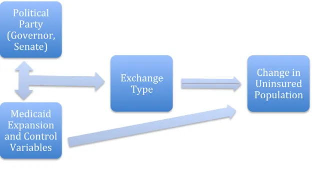
Figure 8: Instrumental Variables Model

In order to address this problem of endogeneity, I propose an instrumental variables

model as a viable alternative approach to OLS regression. While I do not discredit my initial

OLS findings, I believe that it is important to present a different model that addresses the

Political

Party

(Governor,

Senate)

Exchange

Type

Medicaid

Expansion

and Control

Variables

(28)

potential problem of endogeneity. As I have mentioned before, the type of exchange that was

chosen by a state government is often determined by its political party control. Because of the

strong correlation between these two concepts, I propose using the two political party variables

as instruments on the type of exchange. However, before using these variables as instruments, I

must first make sure that they do not have their own unique effects on the dependent variable

(change in uninsured population).

First, I look back at my OLS regression results. In this regression, both the governor and

senate political party variables did not have a significant effect on the change in uninsured

population. From these results, it appears that these variables do not greatly impact the change in

uninsured population directly. After looking at these initial results, I also tabulated the

correlations between the governor’s party (r = -.321) and senate’s party (r = -.231) and found that

the political party variables were not strongly correlated with the change in uninsured population.

Based on these two findings, as well as the strong correlations between political party and

(29)

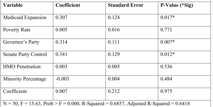
Table 4: “Better Access to Care” IV Model (First Stage)

IV Regression (Dependent Variable: Exchange Type)

Medicaid Expansion 0.307 0.124 0.017*

Poverty Rate 0.005 0.016 0.771

Governor’s Party 0.314 0.111 0.007*

Senate Party Control 0.341 0.129 0.012*

Coefficient 0.007 0.212 0.975

N = 50, F = 15.63, Prob > F = 0.000, R-Squared = 0.6857, Adjusted R-Squared = 0.6418

The first stage of the regression illustrates the reasoning behind using governor’s party

and senate party control as instruments. Along with Medicaid expansion, both the governor’s

party and senate party control are significant at the 95% confidence level. This indicates that they

are effective instruments for determining the exchange type of a state. As I originally predicted,

these two variables are the most important predictors of exchange type. The p-value of the entire

model is also important to note in this situation. At .000, the p-value shows that our instruments

are effective in predicting the outcome of exchange type. Based on these statistics in the first

(30)

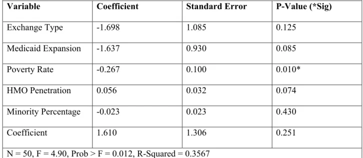
Table 5: “Better Access to Care” IV Model (Second Stage)

IV Regression (Dependent Variable: Percentage Point Change in Uninsured Population)

Exchange Type -1.698 1.085 0.125

Medicaid Expansion -1.637 0.930 0.085

Poverty Rate -0.267 0.100 0.010*

Coefficient 1.610 1.306 0.251

N = 50, F = 4.90, Prob > F = 0.012, R-Squared = 0.3567

The second (and final) stage of the regression reveals important new characteristics about

the independent variables. When viewing the two choice variables, it is evident that neither is

significant at the 95% confidence level. However, both exchange type (p = 0.125) and Medicaid

expansion (p = 0.085) have very low p-values, and appear to contain joint significance. I test this

significance later in the analysis. Based on the negative coefficients of these variables, it appears

that their presence reduced the percentage of uninsured citizens within a state. As for the control

variables, the only one that is significant at the 95% level is the poverty rate of a state. The

coefficient on this variable is negative at -0.267. This indicates that the more impoverished a

state is, the more likely its uninsured population dropped during the first enrollment period. The

other control variables are not significant at the 95% level. However, the managed care

penetration of a state seems to play a role in the model (p = .074). Ultimately, this model

(31)

Table 6: “Better Access to Care” IV Hypothesis Test

Exchange Type, Medicaid Expansion 0.001*

As I already did in the OLS model, it is important to find the direct impact of state

government actions on “better access to care.” Once again, I use a joint significance test to

determine whether or not exchange type and Medicaid expansion have a joint effect on the

change in uninsured population. The results of the test illustrate that the type of exchange and

Medicaid expansion are jointly significant at the 95% confidence level based on the instrumental

variables model. This leads me to reject the hypothesis that, when controlling for other factors,

exchange type and Medicaid expansion have no effect on the change in uninsured population.

Specifically, the coefficients on these two variables (-1.698 for exchange type, -1.637 for

Medicaid expansion) illustrate their marginal effects on the uninsured population. This

conclusion, as well as the magnitude of the coefficient, lends support to my initial hypothesis.

iv. Results/Conclusion

This section includes two unique models to analyze the impact of state government

actions on “better access to care”. While each model presents slightly different numbers, they

both contain very similar results. The OLS model isolates Medicaid expansion as the key factor

in providing “better access to care”. According to the model, states that expanded Medicaid saw

a decrease in uninsured population of 1.95 percentage points more than states that chose not to

(32)

statistically significant in this model, but it was significant when jointly tested with Medicaid

expansion. For the instrumental variables model, neither Medicaid expansion nor exchange

creation was statistically significant on its own. However, the joint significance test showed that

the two state government actions are significant at the 99% confidence level. Both models lead

me to conclude the following result.

Result for Goal 1: In supporting the goal of “better access to care”, I find that states that acted

on exchange implementation or expansion of Medicaid are more likely to have positive results

than those that did not. Specifically, states that expanded Medicaid were most likely to provide

“better access to care” for citizens. However, there is considerable evidence that exchange

(33)

VI. Goal 2: “More Affordable Coverage”

i. Specific Research Design

Dependent Variable: Insurance Premium

The last of the two goals that must be operationally defined is “more affordable

coverage.” To measure the effectiveness of the ACA on affordability, I do a state-by-state

comparison of premium rates (with subsidies included) adjusted for cost of living for similar

plans. It is important to note that this method is slightly different from the method that I use for

“better access to care”. Instead of doing a time comparison for each state’s premium rate, I

compare premium rates across states at a fixed time (2015). I selected this method because I did

not have viable time-series data for premium rate. Using data from the Kaiser Family Foundation

(34)

data on the average price for a bronze plan after tax credits for a 40-year-old non-smoker in

different cities. The specific cities and their individual pricing are presented in the appendix. I do

not include them here for the sake of preserving space. It is important to note that there is exactly

one city for all 50 states. I use the cost of living (Pay Scale 2015, 1) adjustment to observe the

real cost of health care in each area instead of the less meaningful, nominal rate. The probability

density of this variable is presented above in figure nine. It is slightly skewed left, but not

enough to greatly alter the mean.

Control Variables: City Poverty, Managed Care Penetration, Minority Population

Table 7: Bivariate Correlations with Insurance Premium

Variable Correlation Coefficient Significance

City Poverty 0.208 0.147

HMO Penetration -0.129 0.371

Minority Population -0.301 0.034*

For this model, I use the same control variables as I did for the first goal with some minor

adjustments. I keep the model the same because it contains the most relevant predictors of the

insurance market. Because the dependent variable that I use is for cities instead of states, I try to

implement city-level data where available. Unfortunately, I was only able to find comprehensive,

city-level data for poverty (Congressional Research Service 2013, 47), so the other variables

remain unchanged. However, because most of the cities used in this set encompass the majority

of the population in their respective states, I find it appropriate to still use state level data for the

(35)

relevance in determining cost. However, it is included as an instrumental variable in the

instrumental variables model. The correlations for these variables with my independent variable

are presented in table seven.

Summary Statistics

Table 8 (Sources: Gallup-Healthways Well-Being Index, 2014; Kaiser Family Foundation, 2014

2015; U.S. Census Bureau, 2010; Congressional Research Service, 2013)

Variable Mean Standard Deviation

Insurance Premium 120.765 29.197

Exchange Type 0.46 0.50

Medicaid Expansion 0.48 0.50

City Poverty Rate 14.074 3.163

Governor’s Party 0.42 0.50

Senate Party Control 0.40 0.49

HMO Penetration 17.61 11.68

Minority Percentage 28.60 15.48

In table eight, I present the relevant summary statistics for the variables in my model for

“more affordable coverage”. Most of these variables are contained in my original discussion of

the summary statistics for “better access to care”, so I do not discuss them here. Instead, I focus

on the two new variables for this section: insurance premium and city poverty rate. The mean for

insurance rate is 120.765, indicating that the mean premium rate for my given insurance plan and

(36)

idea of the dispersion of premium rates among different cities. As for the city poverty rate, the

mean is at a value of 14.074%. This value is easily compared to the mean poverty rate by state,

which is 12.142%. I expected that the city poverty rate mean would be slightly higher due to the

large concentration of impoverished Americans in cities. The standard deviation of 3.163

indicates a moderate dispersion among city poverty values. While these summary statistics do

not say much on their own, they are important to keep in mind for the next stage of the thesis.

ii. Data Analysis: OLS Regression

Table 9: “More Affordable Coverage” OLS Model

OLS Regression (Dependent Variable: Insurance Premium)

Exchange Type -9.558 9.252 0.307

Medicaid Expansion 3.976 8.582 0.645

City Poverty Rate 2.969 2.094 0.163

Minority Percentage -0.867 0.347 0.016*

Coefficient 101.047 29.471 0.001*

N = 50, Prob > F = 0.012, R-Squared = 0.2074

The OLS regression presents inconclusive results. Based on the p-values for exchange

creation and Medicaid expansion, I cannot draw a conclusion about their individual effect on

(37)

effect on insurance premiums. The same case is true for Medicaid expansion. At the 95%

confidence level, I fail to reject that Medicaid expansion has no effect on insurance premiums.

Despite the lack of meaningful effect for my choice variables, one of my control

variables is statistically significant. At the 95% confidence level, I reject the hypothesis that

minority population has no effect on insurance premiums. Based on its coefficient, I conclude

that an increased level of minorities in a city causes its insurance premiums to decrease. This

finding provides some meaningful information about the insurance market, but it does not

describe a meaningful relationship between state government actions and the goal of "more

affordable coverage". In order to evaluate this relationship in a more complete manner, I turn to a

joint significance test for my two choice variables.

Table 10: “More Affordable Coverage” OLS Hypothesis Test

Exchange Type, Medicaid Expansion 0.575

In this case, the joint significance test is also inconclusive. At the 95% confidence level, I

fail to reject the hypothesis that both exchange type and Medicaid expansion have no effect on

insurance premiums. While these variables are not statistically significant, it is important to view

their coefficients and evaluate them. This regression is especially notable because the two choice

variables seem to work in opposite directions. Exchange type has a negative coefficient,

indicating that states that chose a state exchange are more likely to have lower premiums. I

(38)

positive outcomes for the law. However, the coefficient for Medicaid expansion weakens support

for this assumption. As shown in table nine, the coefficient for Medicaid expansion is positive.

This indicates that states that chose to expand Medicaid tend to have higher insurance premiums.

This coefficient is very notable because it represents a positive state government action resulting

in a negative outcome. This phenomenon requires further analysis, which is done in the second

model for "more affordable coverage". It is important to note that the coefficients for these two

variables are to not be taken as completely relevant, as both variables are not statistically

(39)

iii. Data Analysis: IV Regression

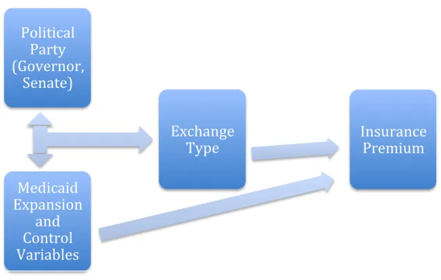
Figure 10: Instrumental Variables Model

The same endogeneity problems exist for the goal of “more affordable coverage” as they

did with “better access to care”. Once again, the problems are with the choice variable of

exchange type. The variable is not randomly assigned but rather highly correlated with the

political party control of a state. For this reason, I use the same instrumental variables method for

the goal of “more affordable coverage”. As visually illustrated in figure 10, this model uses the

political party of the governor and senate as instruments for exchange type. I hope to eliminate

the problem of endogeneity by utilizing this model in this stage of the project.

Political

Party

(Governor,

Senate)

Exchange

Type

Medicaid

Expansion

and

Control

Variables

(40)

Table 11: “More Affordable Coverage” IV Model (First Stage)

IV Regression (Dependent Variable: Exchange Type)

Medicaid Expansion 0.299 0.124 0.020*

Governor’s Party 0.327 0.112 0.006*

Senate Party Control 0.351 0.129 0.009*

Coefficient -0.078 0.219 0.721

N = 50, F = 15.68, Prob > F = 0.000, R-Squared = 0.6888, Adjusted R-Squared = 0.6454

Much like the IV regression for “better access to care”, the first stage of the regression

illustrates the reasoning behind using governor’s party and senate party control as instruments.

The estimates are very similar to the first goal, as only the poverty rate variable is altered to

reflect city-level data instead of state-level. Along with Medicaid expansion, both the governor’s

party and senate party control are significant at the 95% confidence level. This indicates that they

are effective instruments for determining the exchange type of a state. The p-value of the entire

model is also important to note in this situation. At .000, the p-value shows that our instruments

are effective in predicting the outcome of exchange type. Based on these statistics in the first

(41)

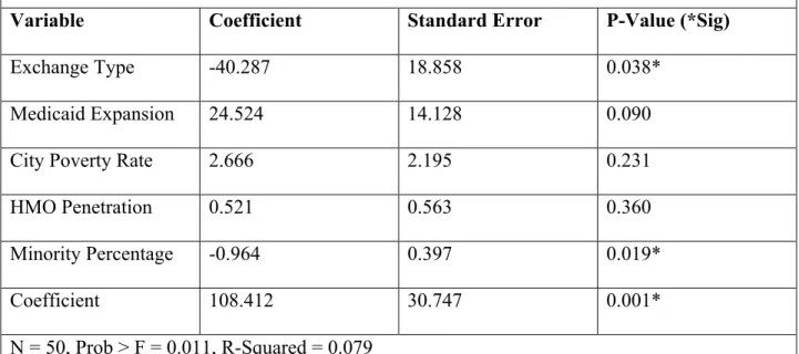
Table 12: “More Affordable Coverage” IV Model (Second Stage)

IV Regression (Dependent Variable: Insurance Premium)

Exchange Type -40.287 18.858 0.038*

Medicaid Expansion 24.524 14.128 0.090

Minority Percentage -0.964 0.397 0.019*

Coefficient 108.412 30.747 0.001*

N = 50, Prob > F = 0.011, R-Squared = 0.079

The IV model presents several notable results. First, as with the OLS model, the minority

percentage is significant at the 95% confidence level. At this level, I reject the hypothesis that the

percentage of minority citizens in a state has no effect on city-level insurance premiums,

controlling for all other factors. This result is consistent with the OLS model, so I generally

expected it to occur. However, for the first time in this analysis, this regression presents a new

result that is not present in the OLS model. According to the IV model, at the 95% confidence

level, I reject the hypothesis that exchange type has no effect on city-level insurance premiums.

The coefficient on this variable indicates that states that chose a state marketplace can expect to

have $40.29 less in insurance premium rates than those that opted for a federal exchange.

This significant result represents a potentially important finding in relation to state

(42)

certain result for two main reasons. The first reason deals with the fact that it contrasts with the

OLS regression results. In the initial regression that I use for “more affordable care”, the

exchange type variable does not approach significance. It exhibits a p-value of 0.307, indicating

that exchange type is not a significant factor in determining insurance premium rates. Because of

this insignificance, I do not consider the significant finding for the IV regression to be certain.

Secondly, I do not consider the IV finding to be completely legitimate because of the

coefficient for Medicaid expansion. Throughout this process, one of my key assumptions has

been that positive state government actions are not detrimental to the implementation of the

Affordable Care Act. However, the coefficient for Medicaid expansion presents a positive state

government actions resulting in a negative outcome for “more affordable coverage”. While I do

not reject the hypothesis that Medicaid expansion has no effect on insurance premiums, it is still

important to recognize that this variable has a negative coefficient. If state government actions

truly have an impact on “more affordable coverage”, I expect that positive actions will result in

positive results. Next, I turn to the joint significance test as another way to test my choice

variables.

Table 13: “More Affordable Coverage” IV Hypothesis Test

Exchange Type, Medicaid Expansion 0.113

The joint hypothesis test for my IV model exhibits the same results as my OLS model. At

(43)

expansion have no effect on insurance premiums. I expected this result, due to the fact that the

two variables work in opposite directions. In this case, the joint p-value is lower than each of the

p-values for exchange type and Medicaid expansion as individual variables. This can be

contributed to the different direction of their coefficients, as mentioned before. While the two

variables are not jointly significant in either model, that does not render the result of this part of

the investigation insignificant. I discuss the broader relevance of these findings in the succeeding

Results/Conclusion section.

iv. Results/Conclusion

This section includes two unique models to analyze the impact of state government

actions on “more affordable coverage”. While each model is designed to present similar

numbers, they contain different results. The OLS model does not isolate either state government

action variable as the deciding factor in “more affordable coverage”. The joint significance test is

also inconclusive, and the variables for exchange type (negative) and Medicaid expansion

(positive) actually work in opposite directions. For the instrumental variables model, I received

slightly different results. In this model, both variables work in opposite directions again. This

time, however, the exchange type is significant. The differing results in each model present

problematic evidence for analyzing the exact effect of state government actions on “more

(44)

Result for Goal 2: In supporting the goal of “more affordable coverage”, I find the exact effect

to be inconclusive for states that acted on exchange implementation or expansion of Medicaid.

The results are inconclusive for two main reasons: conflicting results in my two models, and the

presence of considerable evidence that positive state government actions caused both positive

and negative results for the goal of “more affordable coverage”. Specifically, there is some

support for the hypothesis that state exchange creation caused lower premium rates as indicated

by the IV model (but not the OLS model). But, there is also some support that Medicaid

expansion caused higher premium rates as indicated by the positive coefficients in both models.

Due to these conflicting factors, I am unable to present a conclusive finding for “more affordable

coverage”. While I cannot be sure, this inconclusive finding could potentially indicate that

insurance costs rely more on the private sector than government actions. The government can

only control the structure of the market and encourage competition; it does not have much

(45)

VII. Conclusion

For this analysis, I execute every step of the research process in trying to find a solution

to my initial research question. First, I introduce the reader to the topic and the relevant literature

within this topic. Next, I provide a theoretical model and causal mechanism that underlines my

theory on the topic. In this section, I also hypothesize about the impact of state government

actions on the Affordable Care Act. My hypothesis is that in a comparison of states, those that

set up Affordable Care Act exchanges and/or expanded Medicaid will be more likely to have

positive results than those that did not. Conversely, those that did not set up Affordable Care Act

exchanges and/or expanded Medicaid will be more likely to have negative results than those that

did. I then present a research design that tests my hypothesis. This design focuses on two

specific goals of the ACA: “better access to care” and “more affordable coverage”. After

explaining these goals, I execute two different empirical models for each goal. These models

lead me to several conclusions.

In supporting the goal of “better access to care”, I conclude that states that acted on

exchange implementation or expansion of Medicaid are more likely to have positive results than

those that did not. Specifically, states that expanded Medicaid were most likely to provide “better

access to care” for citizens. In supporting the goal of “more affordable coverage”, I find the exact

effect to be inconclusive for states that acted on exchange implementation or expansion of

Medicaid. The results are inconclusive for two main reasons: conflicting results in my two

models, and the presence of considerable evidence that positive state government actions caused

both positive and negative results for the goal of “more affordable coverage”. Ultimately, I find

hypothesis to be fully supported by my research. While some of the details are conflicting, there

(46)

were more likely to have positive results than those that did not. Conversely, there is also no

doubt that states that did not act on the law were more likely to encounter negative results.

My research presents a very important finding for the health care literature. However, it

also expands beyond this narrow finding. More broadly, it illustrates an important concept for

truly federal laws. When states are required to aid the implementation of a federal law, their

cooperation is important for its success. If a state does not support a law, it can cause some truly

devastating effects for the law’s goals, as indicated by my findings. Despite these important

findings, there is considerable room for other researchers to add to this study and investigate

other important areas.

Specifically, I suggest three expansions/additions. First, it is important for other

researchers that are investigating health care to try other independent variables that they find

intriguing. While I believe my model to be an accurate predictor of the insurance industry, it is

important for other researchers to use other models and come to alternative conclusions. I tested

this model thoroughly and found it to be useful, but other researchers should be able to alter it.

Another valuable extension involves more current data. My analysis mostly focuses on the first

enrollment period and the statistics that stemmed from it. While this represents an important time

for the ACA, it is just as important to study other enrollment periods and how the law develops

over time. I would suggest that other researchers address this development in future studies.

Lastly, I suggest that researchers explore other truly federal laws and how state government

actions affect them. It would be valuable to have another study that describes this phenomenon.

Ultimately, I have presented a comprehensive analysis of the interaction between state

government actions and the Affordable Care Act that has broader implications for federalism.

(47)

VIII. Works Cited

Benjamin, Elisabeth R., Arianne Slagle, and David R. Jones. 2013. “Commentary: Sink or Swim: The State Ground Game Implementing Insurance Exchanges under the Affordable Care Act.” Public Administration Review 73: S47–S48.

Blumenthal, David, and Sarah R. Collins. 2014. “Health Care Coverage under the Affordable Care Act — A Progress Report.” The New England Journal of Medicine 371: 275-281.

Centers for Medicare and Medicaid Services. 2014. “State Effective Rate Review Programs.”

CMS.gov 1.

Congressional Research Service. 2013. “Poverty in the United States: 2013.” Congressional Research Service 47-59.

Dinan, John. 2011. “Shaping Health Reform: State Government Influence in the Patient Protection and Affordable Care Act.” Publius: The Journal of Federalism 41(3): 395–420.

Gallup-Healthways Well-Being Index. 2014. “Change in Percentage of Uninsured by State, 2013 vs. Midyear 2014.” Gallup 1.

Garthwaite, Craig L. 2012. “The Doctor Might See You Now: The Supply Side Effects of Public Health Insurance Expansions.” American Economic Journal: Economic Policy 4(3): 190–215.

Haeder, Simon F., and David L. Weimer. 2013. “You Can’t Make Me Do It: State Implementation of Insurance Exchanges under the Affordable Care Act.” Public Administration Review 73: S34– S47.

Harrington, Scott E. 2010. “U. S. Health-Care Reform: The Patient Protection and Affordable Care Act.” The Journal of Risk and Insurance 77(3): 703–8.

Hofer, Adam N., Jean Marie Abraham, and Ira Moscovice. 2011. “Expansion of Coverage under the Patient Protection and Affordable Care Act and Primary Care Utilization.” The Milbank

Quarterly 89(1): 69–89.

Jacobs, Lawrence R. 2010. “What Health Reform Teaches Us about American Politics.” PS: Political Science and Politics 43(4): 619–23.

Jacoby, Jeff. 2014. “Mass. model of health care: Wait for it.” Boston Globe. 1.

Joondeph, Bradley W. 2011. “Federalism and Health Care Reform: Understanding the States’ Challenges to the Patient Protection and Affordable Care Act.” Publius 41(3): 447–70.