A novel bi-level stochastic programming model for supply chain
network design with assembly line balancing under demand
uncertainty
Nima Hamta1*, M. Akbarpour Shirazi2 , Sara Behdad3, Mohammad Ehsanifar4 1
Department of Mechanical Engineering, Arak University of Technology, Arak, Iran
2
Department of Industrial Engineering, Amirkabir University of Technology (Tehran
Polytechnic), Tehran, Iran 3
Department of Industrial and Systems Engineering, University at Buffalo, The State University of New York, USA
4
Department of Industrial Engineering, Islamic Azad University of Arak, Arak, Iran
[email protected], [email protected], [email protected], [email protected]
Abstract
This paper investigates the integration of strategic and tactical decisions in the supply chain network design (SCND) considering assembly line balancing (ALB) under demand uncertainty. Due to the decentralized decisions,a novel bi-level stochastic programming (BLSP) model has been developed in which SCND problem has been considered in the upper-level model, while the lower-level model contains ALB problem as a tactical decision in the assemblers of supply chain network. To deal with demand uncertainty, a scenario generation algorithm has been proposed within the stochastic optimization model that combines time series model, Latin hypercube sampling method and backward scenario reduction technique. In addition based on the special structure of the model, a heuristic-based solution method is proposed to solve the developed BLSP model. Finally, computational experiments on several problem instances are presented to show the performance of the model and its solution method. The comparison between the stochastic and equivalent deterministic model demonstrated that the developed stochastic model mainly performs better than the deterministic model especially in making strategic decisions while the deterministic model works better in making tactical decisions.
Keywords: Bi-level stochastic programming, supply chain network design, scenario-based approach, assembly line balancing, uncertain demand
*Corresponding author.
ISSN: 1735-8272, Copyright c 2017 JISE. All rights reserved
Journal of Industrial and Systems Engineering
Vol. 10, No. 2, pp 87-112 Spring (April) 2017
88
1- Introduction
Supply chain network design (SCND) problem is an important issue in supply chain management (SCM) which has attracted research attention over the last few decades. In general in this problem, the optimal number and configuration of the facilities is determined in addition to the quantities of required raw materials, production, distribution and transportation among the facilities such that the customer demand is satisfied and the supply chain value is optimized (Simchi-Levi et al., 2004).
In SCM, there are three levels of decision-making during the time horizon categorized as strategic level (long-term decisions), tactical level (mid-term decisions) and operational level (short-term decisions) (Vidal and Goetschalckx, 1997).The strategic level commonly relates to the decisions such as the determination of number, location and capacity of the facilities and technology selection (Ghiani et al., 2004). SCND is one of the main strategic decisions that sometimes entitled as strategic supply chain planning (Chopra and Meindl, 2007).In the tactical decisions, production levels at manufacturers/factories, assembly policy, lot sizes and inventory levels are determined. Finally, the operational level deals with the scheduling of material flows based on the decisions made in two upper levels (Schmidt and Wilhelm, 2000).
Recently, several review papers have been published on SCND area. Shen, (2007) presents a survey on the new developments of integrated SCND optimization models, especially nonlinear models. Akyuz and Erkan (2010) provide a review on performance measurement of supply chains. They present the basic research approaches and methodologies, requirements and areas for the performance management of the recent supply chain era. Melo et al., (2009) review facility location models in the SCM context and basic features these models must capture to support decision making in the design of supply chain networks across different industries. Klibi et al., (2010) review the optimization models proposed for the SCND problem under uncertainty. They also investigate related strategic SCND evaluation criteria and their use in the existing models. Very recently, Martínez and Moyano (2014), have evaluated the state-of-the-art researches into the relations between SCM, lean management and sustainability to identify the studied areas and the orienting future research.
Many mathematical models have been developed in the related literature in order to design and optimize the supply chain networks (SCNs) by now. These models can range from simple uncapacitated single-product facility location models (see for example Sung and Song, (2003)) to complex capacitated multi-commodity models (see for example Tsiakis and Papageorgiou (2008)) with different objectives such as total cost minimization or profit maximization. Most of these models concentrate on the transportation/distribution networks with considerations such as facility location, capacity planning, inventory management, vehicle routing and so on (Paksoy and Özceylan, 2012a).
In the recent studies, the SCND problem under uncertainty has received much attention and the literature related to this issue is considerably increasing (Klibi et al., 2010). Many studies have addressed customer demand as the only uncertain parameter. Longinidis and Georgiadis (2011) present a mathematical model as an effective strategic decision tool to integrate SCND decisions with financial statement analysis under demand uncertainty. Hamta et al., (2014) investigate the optimization of strategic and tactical decisions in a SCND problem under demand uncertainty. Furthermore, some studies consider several stochastic parameters simultaneously. In this regard, Pishvaee et al.,(2009) develop a stochastic mixed-integer linear programming (SMILP) model for multi-stage logistics network design in which quantity and quality of returned products, demands and variable costs are uncertain parameters. Mohammadi Bidhandi and Mohd Yusuff (2011) state that uncertainty generally finds in tactical decisions because most of the tactical parameters are not totally certain when strategic decisions are made. They consider customer demand, capacity of the facilities and operational costs as uncertain parameters.
The production system is one of the vital factors for the optimization of SCNs. In order to create an efficient SCN involved with assembly activities, two main functions of supply chain such as transportation and assembly line processes must be integrated appropriately (Paksoy et al., 2012b). This integration has two main aspects for a supply chain. Firstly, companies try to obtain maximum value by minimizing the transportation costs at each stage of the supply chain. Secondly, companies attempt to optimize the operations inside the supply chain such as line balancing and the opening costs of workstations. Therefore, there is a relationship between logistics processes and assembly line processes that necessitates the integration between them in the SCN (Paksoy and Özceylan, 2012a). On the other hand, assembly line balancing (ALB) as one of the decisive factors, is the most common
89
operation in SCNs especially when there are a lot of components. It is worth mention that an assembly line consists of a set of sequential workstations connected by a material handling system. In each workstation, a set of tasks is performed while each task has a certain processing time and there is a pre-defined precedence diagram, which determines the sequence of performing the tasks (Becker and Scholl, 2006). In this regard, the main objective of the ALB problem is to assign a set of tasks to the workstations in such a way that the precedence constraints among tasks are met and some measures, such as number of workstations, cycle time or line efficiency are optimized (Hamta et al., 2013). Since balancing the assembly activities has significant influence on the performance and productivity of systems, optimizing assembly activities affects the SCN performance. Many companies such as automobile companies are confronted with this problemwhere logistics processes and assembly line activities should be considered concurrently tolead to better performance in terms of customer satisfaction, reliability and agility (Hamta et al., 2014).
The importance of uncertainty modeling in different decision levels of SCND has motivated a number of researchers to use stochastic programming approaches when one or more uncertain parameters or variables exist in the optimization problem (see for example Pishvaee et al., (2009) and Santoso et al., (2005)). Schütz et al., (2009) develop a two-stage stochastic program to formulate a multi-commodity SCND problem with a description of operational consequences from the strategic decisions. They address strategic location decisions in the first stage decisions and operational decisions in the second-stage. Hamta et al., (2014) propose a two-stage stochastic programming model in which the first-stage contains strategic location decisions, while in the second-stage the SCND and ALB decisions are made.
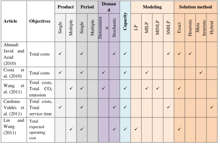
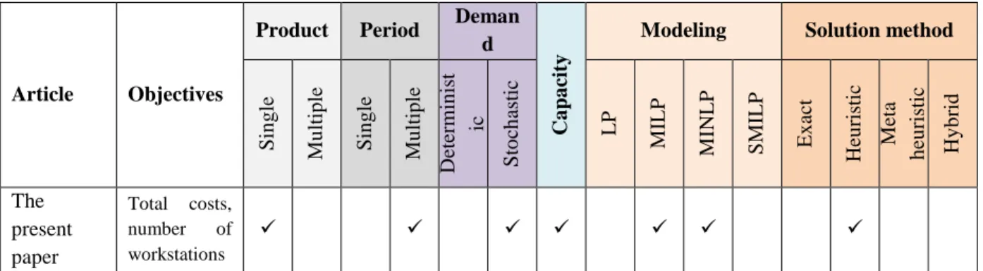
Table 1 presents a detailed classification of the recent papers published after 2010 based on some supply chain characteristics and decisions such as objectives, characteristics of product and period, uncertainty in demand, capacity, type of modeling, and the solution method. The characteristics of our problem in this paper have been stated in the last row of Table 1. It is worth mentioning that the papers reviewed in Table 1 have been selected based on the similarity to our work in terms of characteristics such as modeling approach and basic assumptions.
Table 1.The supply chain decisions of recent papers in SCND arae
Article Objectives
Product Period Deman d C a p a ci ty
Modeling Solution method
S in g le M u lt ip le S in g le M u lt ip le D et er m in is t ic S to ch as ti c L P M IL P M IN L P S M IL P E x ac t H eu ri st ic M et a h eu ri st ic H y b ri d Ahmadi Javid and Azad (2010)
Total costs
Costa et
al. (2010) Total costs Wang et
al. (2011)
Total costs, Total CO2
emission
Cardona-Valdés et al. (2011)
Total costs, Total service time Lin and
Wang (2011) Total expected operating cost
90 Article Objectives
Product Period Deman d C a p a ci ty
Modeling Solution method
S in g le M u lt ip le S in g le M u lt ip le D et er m in is t ic S to ch as ti c L P M IL P M IN L P S M IL P E x ac t H eu ri st ic M et a h eu ri st ic H y b ri d Georgiadis et al. (2011)
Total costs
Rezapour et al. (2011) Profit Longinidis and Georgiadis (2011) Economic value added
Nickel et al. (2012) Total financial benefit Sadjady and Davoudpo ur (2012) Total costs
Tsao and
Lu (2012) Total costs Babazadeh
et al.(2012)
Total costs
Melo et al.
(2012) Total costs Paksoy et
al. (2012c)
Total transportatio n costs
Carle et al. (2012)
Net operating profits Singh et
al. (2013)
Total (expected) costs Vahdani et
al. (2013) Total costs Kristianto
et al. (2014) Inventory and transportati on Khalili-Damghani (2014) Total purchasing cost Roni et al.
(2014) Total costs
91 Article Objectives
Product Period Deman d C a p a ci ty
Modeling Solution method
S in g le M u lt ip le S in g le M u lt ip le D et er m in is t ic S to ch as ti c L P M IL P M IN L P S M IL P E x ac t H eu ri st ic M et a h eu ri st ic H y b ri d The present paper
Total costs, number of workstations
LP: Linear Programming; MILP: Mixed-Integer Linear Programming; MINLP: Mixed-Integer Nonlinear NLP: Non Linear Programming
Although SCND problem has been investigated widely, but little attention has been given to use bi-level programming (BLP) as the modeling approach. SCND problem can be considered as a Leader-Follower where top managers are the leaders, and the assemblers are the followers who make decisions about their activities considering top-level decisions Hamta et al., (2015). Roghanian et al., (2007) propose a probabilistic multi-objective BLP problem and its application in enterprise-wide supply chain planning where some parameters are random variables. Sun et al. (2008) developed a BLP model to obtain the optimal location of distribution centers where the upper-level model determines the optimal location, and the lower-level model gives an equilibrium demand distribution.
The main contribution of this paper is to develop a bi-level stochastic programming (BLSP) for a SCND problem considering ALB and demand uncertainty. To the best of authors’ knowledge, this problem which is applicable to many real-world situations, is novel and has not been addressed in the related literature. The most similar study to our work belongs to Paksoy et al., (2012b). They developed an MINLP model to integrate SCND and ALB problems. However, they did not pay attention to the bi-level nature of the problem. In addition, since the variations in customers’ demands change the products shipped between layers of the SCN in each period, demand uncertainty has significant effects on the flows inside the SCN. This issue also affects the assignment of tasks and layout of the workstations. The main objective of the developed BLSP model in this paper is to optimize the performance of the considered SCN under demand uncertainty. A scenario-based algorithm is proposed to deal with demand uncertainty in which time series model and Latin hypercube sampling (LHS) (Iman, 2008) are employed. Finally, the BLSP model performance is evaluated under generated scenarios.
The remainder of this paper is structured as follows. Section 0introduces problem description and mathematical formulation of the BLSP model under study. Section 0 explains how to deal with demand uncertainty that serve as input to developed BLSP model. Section 0describes the solution method. The computational experiments over several problem instances and the comparison with the deterministic model are presented in Section 0. Finally, Section 0 leads to the concluding remarks and guidelines for future research.
2- Problem statement and formulation
In this section, the problem statement, notations and the mathematical formulation of problem under study are presented.
2-1- Problem statement
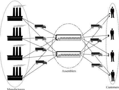
This paper considers the simultaneous optimization of strategic and tactical decisions in the SCN to design and optimize an SCN. Figure 1 shows the structure of considered SCN including manufacturers, assemblers and customers. An SCND problem is addressed as a strategic decision and ALB problem is tackled as a tactical decision. In the assemblers, single-product and straight assembly lines are concerned with the aim of minimizing the number of workstations for a certain cycle time.
The main purpose of this paper is to model and solve an SCND problem considering ALB using stochastic BLP. BLP is a tool to model decentralized decisions which contains the objective(s) of the leader at the first level and that of the follower at the second level (Colson, 2005). Since the problem
92
under study involves two different decision-makers including supply chain managers and the assemblers’ decision makers who make connected decisions with interactions on each other, BLP is adapted to describe the problem appropriately (Hamta et al., 2015).Considering demand uncertainty, the problem is formulated as a BLSP model in which SCND problem as a strategic decision is considered in the upper-level model, while the lower-level model contains the ALB as a tactical decision. The main decision variables obtain after solving the model are the amount of flows between two sequential echelons, assemblers’ cycle times, and tasks assignment to the workstations in the assemblers.
Figure 1. The structure of considered SCN
The basic assumptions behind the studied problem are common assumptions for SCND and ALB problems (see for example Hamta et al., (2014)). In this paper, it is assumed the maximum capacity of manufacturers and assemblers is given. In addition, the upper bound of the number of potential workstations at each period is determined via dividing total task times by average initial cycle times. 2-2- Mathematical model
This subsection presents the BLSP formulation of the problem. The scenario-based stochastic approach has been used in the BLSP model for capturing the customers’ demands in both levels of the model to find the best decisions. The proposed scenario-based approach will be explained in Section 0 in detail.
2-2-1-Basic model of BLSP
A BLP model is applied for a problem with two different decision-makers, which make decentralized decisions successively (Colson, 2005). In this paper, supply chain network decisions such as flows of products and cycle times are made by top-level managers, and then determined decisions are employed in assemblers to balance the assembly lines. Since we concern uncertainty in customers’ demands, a stochastic version of BLP has been used in the paper. BLSP method allows applying concepts of stochastic programming directly to bi-level structure. In other words, BLSP completes relationship between the actors to deal with bi-level structure and uncertainty simultaneously. The stochastic programming framework seems more flexible and investigations connected with the bi-level structure can be incorporated more efficiently into the stochastic programming context (Werner, 2005). Therefore, the BLSP approach can treat the implications of the bi-level features adequately.
In terms of BLSP, a general stochastic programming problem with bi-level structure can be formulated as follows where the uncertainty environment is expressed by a random variable ω∈Ω. In
93
addition x and y are the decision variables of upper-level and lower-level problems, respectively (Werner, 2005):
* *
(U) Min ( , , ) . . ( , , ) 0,
x F x y
s t G x y
ω
ω
≤(1)
where y*is an optimal solution of the leader’s perception of the follower’s decision process. (L) Min ( , , )
. . ( , , ) 0
y f x y
s t g x y
ω
ω ≤ (2)
The BLSP model consists of two sub-problems: (U) is an upper-level problem with variables
1 n
x ∈R and (L) is a lower-level problem with the decision vector of the lower-level decision-makers
2 n
y∈R . Function F:Rn1×Rn2× Ω →R is the objective function of upper-level decision-makers or
top-level managers, and the vector-valued function G R: n1×Rn2× Ω →Rm1is the constraint set of the
upper-level decision vector. Similarly, function f :Rn1×Rn2× Ω →R is the objective function of
lower-level decision-makers, and g R: n1×Rn2×Ω →Rm2 is the constraint set of the lower-level
decision vector. All of the constraints and objective functions may be linear, quadratic, nonlinear, fractional, etc.
2-2-2- Model notations
The sets, indices, constants, parameters and decision variables employed in the mathematical model are defined as follows:
Sets and indices:
M set of manufacturers, indexed by m∈M
A set of assemblers, indexed by a∈A
C set of customers, indexed by c∈C
J set of potential workstations with estimated number of potential workstations, indexed by j∈J
N set of tasks, indexed by i∈N
r, q index of tasks
P set of couples of tasks (r, q) in which task r is the immediate predecessor of task q
K set of components ,indexed by k∈K
T set of periods in planning horizon, indexed by t∈T
S set of scenarios, indexed by s∈S
Constants and parameters:
MA mat
TC transportation cost from manufacturer m to assembler a at period t
AC act
TC transportation cost from assembler a to customer cat period t MA
ma
Dc distance between manufacturer m and assembler a AC
ac
Dc distance between assembler a and customer c M
mkt
Cap capacity of manufacturer m for component k at period t A
at
Cap capacity of assembler a at period t cts
D demand of customer c at period t in scenario s
i
t task time of task i
Prts occurrence probability of scenarios at period t t
94 Decision variables:
MA makts
Y Quantity of component k shipped from manufacturer m to assembler a at period t in scenario s AC
acts
Y quantity of product shipped from assembler a to customer c at period t in scenario s if task is assigned to workstation for assembler at period in scenario
1 ,
otherwise 0
aijts
i j a t s
V =
if at least one task is assigned to workstation for assembler at period in scenari
1 o ,
otherwi
0 se
ajts
j a t s
Z =
ats
CT cycle time for assembler aat period t in scenario s
2-2-3- Upper-level model
In the upper-level of our developed BLSP model, the considered SCND decisions are made including the amount of flows between two sequential echelons and assemblers’ cycle times under demand uncertainty.
Pr
Min ts matMA maMA maktsMA actAC acAC actsAC
t T s S m M a A k K a A c C
U TC Dc Y TC c
Z D Y
∈ ∈ ∈ ∈ ∈ ∈ ∈ = × × × + × ×
∑∑
∑ ∑ ∑
∑∑
(3)MA M makts mkt a A Y Cap ∈ ≤
∑
∀ ∈m M,∀ ∈k K,∀ ∈ ∀ ∈t T, s S (4)AC A acts at c C Y Cap ∈ ≤
∑
∀ ∈ ∀ ∈ ∀ ∈a A, t T, s S (5)AC acts cts a A Y D ∈ ≥
∑
∀ ∈ ∀ ∈ ∀ ∈c C, t T, s S (6)0
MA AC
makts acts m M c C
Y Y
∈ ∈
− =
∑
∑
∀ ∈ ∀ ∈a A, k K,∀ ∈ ∀ ∈t T, s S (7)A C ats t acts
c C
CT W T Y
∈
≤
∑
∀ ∈ ∀ ∈ ∀ ∈a A, t T, s S (8), , 0
MA AC makts acts ats
Y Y CT ≥ ∀ ∈m M,∀ ∈ ∀ ∈a A, k K,∀ ∈ ∀ ∈ ∀ ∈t T, c C, s S (9)
The objective function of upper-level model, i.e. Relation (3), minimizes the expected transportation costs between two sequential echelons. Constraints (4) and (5) assure the total quantity of components shipped from each manufacturer to the assemblers, and the total amount of products shipped from each assembler to the customers should not exceed the capacity of that manufacturer and assembler at each period in each scenario, respectively. Constraint (6) guarantees the satisfaction of customer demand for all products at each period in each scenario. Relation (7)shows the total component amount shipped from manufacturers to the assembler equals to the total shipped product amount from that assembler to customers to satisfy the demand at each period in each scenario. Constraint (8) states that cycle time of all assemblers at each period in each scenario must be lower than or equal to the working time in all periods divided by the total product amount shipped from each assembler to customers. Constraint (9) denotes the non-negativity restriction of upper-level decision variables, i.e.
MA makts
95
2-2-4-Lower-level model
The lower-level of our developed BLSP model represents the assignment of tasks to the workstations in the assemblers, which is the objective of ALB problem. It should be noted that the simple assembly line balancing problem (SALBP) is categorized into two main groups: SALBP-I and SALBP-II. SALBP-I intends to assign tasks to the workstations in such a way that the number of workstations is minimized for a given cycle time, while SALBP-II tries to minimize the cycle time for a given number of workstations (Hamta et al., 2011).Since SALBP-I generally happens when the organization intends to design new assembly lines, we select this type which is more compatible with the considered problem in the lower-level model.
Min Prts ajts
t T s S a A j J t T
L Z
Z
∈ ∈ ∈ ∈ ∈
= ×
∑∑
∑∑∑
(10)1
aijts j J
V ∈
=
∑
∀ ∈ ∀ ∈a A, i N,∀ ∈ ∀ ∈t T, s S (11)0
arjts aqjts
j J j J
j V j V
∈ ∈
× − × ≤
∑
∑
∀ ∈ ∀a A, ( , )r q ∈ ∀ ∈ ∀ ∈P, t T, s S (12)i aijts ats i N
t V CT
∈
× ≤
∑
∀ ∈ ∀ ∈ ∀ ∈ ∀ ∈a A, j J, t T, s S (13)aijts ajts i N
V M Z
∈
≤ ×
∑
∀ ∈ ∀ ∈ ∀ ∈ ∀ ∈a A, j J, t T, s S (14), {0,1}
aijts ajts
V Z ∈ ∀ ∈ ∀ ∈a A, i N,∀ ∈ ∀ ∈ ∀ ∈j J, t T, s S (15)
The objective function of lower-level model minimizes the expected total number of opened workstations in all assemblers. Constraint (11) guarantees that each task must be assigned to one workstation in all assemblers at each period in each scenario. Constraint (12) ensures the precedence relations between the tasks by assigning task r as an immediate predecessor of task q in all assemblers at each period in each scenario. Constraint (13) expresses that total task times in each workstation should not exceed the corresponding cycle time in all assemblers at each period in each scenario. Constraint (14) guarantees that workstation j is opened, i.e. Zajts =1, if at least one task is assigned to it in all assemblers at each period in each scenario. Constraint (15)denotes the binary nature of variables Vaijtsand Zajts.
3- Dealing with Demand uncertainty
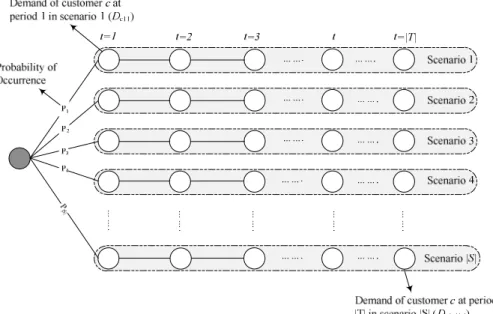
To deal with demand uncertainty, this paper presents a scenario-based approach to generate demand scenarios in the BLSP model by approximating the stochastic demand process fitted from historical data. It is worth mentioning that a scenario is a description of a future state with a probability assigned to it that indicates the importance of that scenario in uncertain environment (Birge and Louveaux, 2011).A scenario tree is employed to represent demand uncertainty with a given probability for each scenario (Figure 2). Each scenario determines the customer’s demand for a certain product in planning horizon. Several demand scenarios are generated from the particular distribution through scenario generation algorithm presented in this section. This algorithm includes three steps, namely time series forecast modeling, LHS method to generate error term in the forecast model, and demand scenario reduction to build the scenario tree from historical data. Details of each step are explained in the following subsections. Figure 3 demonstrates the outline of the proposed scenario generation algorithmtodeal with demand uncertainty in the considered problem.
96
Figure 2.A scenario tree for a customer (c) with discrete demand scenarios
Figure 3.The outline of proposed algorithm for dealing with demand uncertainty and scenario generations
3-1- Time series forecast model
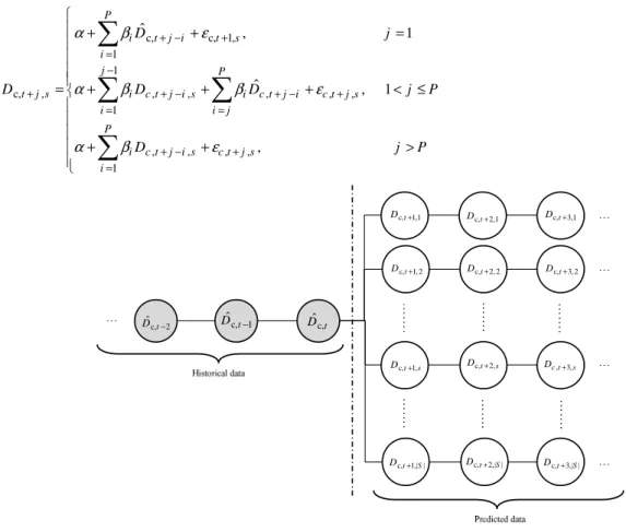
In order to deal with uncertainty, a suitable time series model can be utilized to consider time dependencies of demand in multiple periods in each scenario. We employ an autoregressive (AR) process of P th order to model demand uncertainty(see for example [22]). In our case, the predicted demand at period t + 1 and scenario s denoted byDc,t+1,sconsidering the error termεc, 1,t+s is given by
the following relation:
c, 1, c, c, 1,
1
ˆ
P
t s i t j i t s i
D + α βD + − ε +
=
= +
∑
+ ∀ ∈ ∀ ∈ ∀ ∈c C, t T, s S (16)where α is a constant, βi is AR parameters,Dˆc,t+ −1 iis the historical demand of customer cat (t+ 1– i)
period, andεc, 1,t+ sis the error term at(t + 1) th period and s th scenario. Then, the following formulation
97
c, c, 1, 1
1
c, , , , , , ,
1
, , , ,
1
ˆ , 1
ˆ , 1
, P
i t j i t s
i
j P
t j s i c t j i s i c t j i c t j s
i i j
P
i c t j i s c t j s i
D j
D D D j P
D j P
α β ε
α β β ε
α β ε
+ − +
= −
+ + − + − +
= =
+ − +
=
+ + =
= + + + < ≤
+ + >
∑
∑
∑
∑
(17)
c,
ˆ
t
D
c,t1,s
D + Dc t,+3,s c,t1,1
D + Dc,t+2,1 Dc,t+3,1
c,t1, 2
D + Dc,t+2, 2 Dc,t+3, 2
c,t1,| |S
D + Dc,t+2,| |S Dc,t+3,| |S c, 2
ˆ
t
D − Dˆc,t−1
c,t 2,s
D +
Figure 4.Demand generation method for customer c
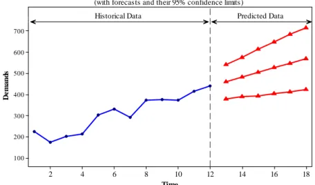
Figure 4 demonstrates a schematic view of generating different scenarios for customer c. The scenarios are generated based on the error terms, which follows normal distribution with mean zero and varianceσε2. In our case, the error terms are generated at each period for all customers based on the method will explain in Subsection 0.As a practical example of implementing the considered time series model, the demand of a special type of civil aircrafts is concerned. Since the historical data has a non-constant mean and variance, therefore the ARIMA model is the most suitable to describe the behavior of demands (Chen and Lu, 2012). For this purpose, first the autocorrelation between data should be checked to help determine a likely model. We performed that and found there is a single large spike of 0.7 at lag 1, which is typical of an autoregressive process of order one (Figure 5).Figure 6showsthe historical data from 2002, i.e. period 1 in the abscissa of Figure 6, to 2013, i.e. period 12 in the abscissa of Figure 6,used to predict the future demands, including the average and 95%confidence intervals of demand values in next 6 months (from period 13 to period 18). Consequently, the estimated ARIMA parameters and the results of related hypothesis test for this product are as follows: Type Coef. SE Coef. T P
AR 1 -0.4482 0.2923 -1.53 0.080 Constant 31.35 12.44 2.52 0.033
98
Figure 5. Autocorrelation Function for demands with 5% significance limits.
Figure 6.Historical and predicted demand quantities of the considered product.
It should be noted that the coefficients of the fitted ARIMA model are estimated by maximum likelihood estimation (MLE) via Minitab statistical software. The mean demand and95% confidence limits (CL) of the considered product based on the fitted model are reported in Table 2for 6 future periods.
Table 2. The mean demand and 95% confidence limits of the productfor 6 periods.
Period 13 14 15 16 17 18
Mean Demand 460.145 482.466 503.812 525.595 547.182 568.857
95% Lower CL 379.259 390.081 393.17 402.652 411.725 422.508
95% Upper CL 541.032 574.852 614.454 648.538 682.639 715.205 3-2- Error term generation using LHS method
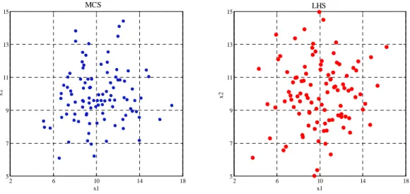
Most of former works have used Monte Carlo simulation (MCS) to generate error term (ε)and consequently different scenarios (See for example Chen and Lu (2012)). In this paper, LHS method is employed to cover more domain space of stochastic parameters rather than MCS. LHS is recommended as a method to improve the efficiency of sampling method (Iman, 2008). Figure 7compares the performance of MCS and LHS methods for an example with two variables x1 andx2following normal distribution (
2 2
1~ (10, 5 ) and 2~ (10,2 )
x N x N ).
6 5
4 3
2 1
1.0 0.8 0.6 0.4 0.2 0.0 -0.2 -0.4 -0.6 -0.8 -1.0
Lag
A
u
to
co
r
re
la
ti
o
n
18 16 14 12 10 8 6 4 2
750 700
600
500
400
300
200
100
Time
D
e
m
a
n
d
s
Time Series Plot for Demands
(with forecasts and their 95% confidence limits)
99
Figure 7. Comparison between LHS and MCS methods.
To construct scenario tree, suppose we have |T| periods. In each period, the error terms are generated using a normal distribution as mentioned before. Since error terms are period-independent, the new terms are generated at the next period by the same way. This procedure is continued until the last period. The steps of LHS method employed to generate error terms are explained in pseudo-code of proposed scenario generation algorithm presented at the end of this section.
3-3- Scenario reduction
As it is clear, large number of scenarios makes the optimization model cumbersome to be solved, especially in large scale problems. In order to reduce the number of scenarios efficiently, a scenario reduction technique should be used. In the literature, two scenario reduction methods exist: backward and forward (Dupačová et al., 2003). For simplicity, we employ backward reduction technique. The
algorithmic framework of backward technique is described in Step 3 of scenario generation algorithm. In the civil aircraft case, the backward reduction algorithm has been used to reduce 80 generated scenarios to 30 reduced set for 3customers in 6 future periods (Figure 8). As shown in the reduction results, the shape and characteristics of generated scenarios are retained and the reduced scenarios can be used to predict appropriately.
2 6 10 14 18
5 7 9 11 13
15 MCS
x1
x
2
2 6 10 14 18
5 7 9 11 13
15 LHS
x1
x
100
(a) (b)
Figure 8.(a) 80 generated scenarios for three customers in six future periods (b) 30 demand scenarios
obtained by reduction method from 80 generated scenarios in (a).
Pseudo-code of the proposed scenario generation algorithm is represented as follows:
Nomenclature:
|S| number of generating scenarios at each period |S|target desired number of reduced scenarios
|C| number of customers
t
Sc set of scenarios at period t
,
Prt jprobability of constructed scenario j at period t
t
DSc set of scenarios that to be deleted at period t
ijt
Dis Euclidean distance between scenario i and j at period t
Begin
For each t∈T
Step 1.Generateεcts(c=1, 2,...,|C|;s=1, 2,...,|S|) using LHS as follows[52]:
i. M is a |C |×|S |matrix in which rows are random permutation of 1,...,|S|.
ii. M′is a |C |×|S |matrix randomly generated using uniform (0,1) distribution.
iii. 1 ( )
| |
G M M
S ′
= − .
iv. ˆ 1( ) ( 1, 2,...,| |; 1,2,...,| |)
itj Fε Gij i C j S
ε = − = = , where 1
()
Fε− is inverse cumulative distribution
1 2 3 4 5 6
400 450 500
550 Customer 1
1 2 3 4 5 6
400 450 500
550 Customer 2
1 2 3 4 5 6
400 450 500
550 Customer 3
Period
1 2 3 4 5 6
400 450 500
550 Customer 1
1 2 3 4 5 6
400 450 500
550 Customer 2
1 2 3 4 5 6
400 450 500
550 Customer 3
101 function of ε.
Step 2.Construct demand scenarios If (t>1)then
a. Construct set Sct by |S| |× S|targetScenarios using Relation (17) using ( 1, 2,...,| |; 1, 2,...,| |)
cts c C s S
ε = = .
b. ,
1
Pr ,
| |
t j
S =
Else
a. Construct |S| demand scenarios for period 1 using Relation (16).
b. 1,
1
Pr , 1,...,| |
| |
j j S
S
= =
End if
Step 3.Backward scenario reduction
i. DefineSctas a set of all initial scenarios at period t and DSctis a null set. ii. While (|Sct | |>S|target)
a.
(
)
| |
2
1 1
, 1,...,| |; 1,...,| |
C t
ijt rpi rpj t t
r p
Dis D D i Sc j Sc
= =
= − = =
∑∑
b.
1,...,| |
min { } 1,...,| |,
t
st ss t t
s Sc
MDis Dis ′ s Sc t T
′=
= ∀ = ∀ ∈ , find the scenario index f that has the
minimum distance with scenario s.
c. CalculatePSst =Prs×MDisst ∀ =s 1,...,|Sct|,∀ ∈t T
d. Find the scenario index d such thatPSdt =minPSst ∀ =s 1,...,|Sct|,∀ ∈t T
e. Sct=Sct−scenario ( ),d DSct=DSct+scenario ( ), Prd t f, =Prt f, +Prt d,
End while End for
End
4- Solution method
It is generally difficult to solve the BLP problem. One reason is that BLP even in its simplest version is an NP-hard problem (Ben-Ayed et al., 1988). Even if both upper and lower-level problems are convex, the whole BLP problem can be non-convex. Therefore, even if we obtain the solution of BLP, it is generally local optimum not global. Finding the response or reaction relation is the key point to solve the BLP. Response relation determines the relationship between upper and lower variables in a BLP model[44]. In the special formulation of this paper, finding relationship between upper-level variables and lower ones is simple. Constraint (13) represents explicitly the relationship between binary lower-level variables and continuous upper-level variables.
Our proposed solution method is a heuristic algorithm based on Constraint (13) by considering the generated demand scenarios using the algorithm presented in Section 0. It should be mentioned that the proposed solution method is a hybrid method in which exact methods have been employed through a heuristic approach. Exact methods such as branch and bound have been implemented by GAMS solvers. In this method, cycle time (CTats) is a given parameter in the lower-level model. After
solving the lower-level model and obtaining the value of variable Vaijts, Constraint (13)should be
added to the upper-level model. Then for the fixed Vaijts obtained from lower-level model, upper-level
problem is solved to find new CTats. This iterative process is continued until the stopping criterion is
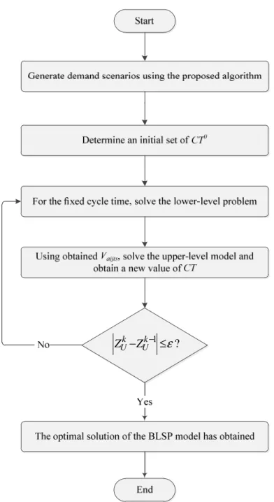
established and convergence to the optimal solution of the original BLSP model. The stopping criterionis that difference betweentwo sequential objective function values of upper-level model should be lower than a small positive number (ε). Following the proposed solution method for the developed BLSP model is presented:
102
Step 1.Generate demand scenarios using the proposed algorithm in Section 0; Step 2.Determine an initial set forCT0;
Step 3. For the fixed CTatsk , solve the lower-level model and obtain Vaijtsk ;
Step 4. Using obtained Vaijtk from Step 3, solve the upper-level model and find a new value for CT;
Step 5. If ZUk −ZUk−1 ≤εstop, where ε is the convergence tolerance; otherwise, set k=k + 1 and go back to Step 3.
Figure 9 shows the steps of the proposed algorithm to solve the considered BLSP model. It should be noted that since upper-level model is an MINLP problem, an appropriate solution method should be employed in iterations such as branch-and-bound method or outer approximation algorithm. Sometimes an inner penalty function method can be utilized to relax nonlinear constraints, and then the upper-level model can be solved by the solution methods of linear convex optimization problems (Roghanian et al., 2007). On the other hand, the MILP solution methods can be employed to solve the level model. In this regard, GAMS/ Cplex as a well-known GAMS solver is used in the lower-level model to obtain optimal solution. Since our proposed solution method is a heuristic method, it is hard to test its convergence. For this purpose, different initial points can be considered to solve the problem and if all results are the same, it shows that the algorithm converges (In this regard, see for example Hamta et al. (2015) and Sun et al. (2008)).
103
1 ?
k k
U U
Z −Z − ≤ε
Figure 9. The steps of the proposed algorithm to solve the developedBLSP model
5- Computational experiments
In order to evaluate the performance of the developed BLSP model and the solution method, numerical experiments over some randomly generated problem instances are used. These instances have been generated in different sizes (small, medium and large) to evaluate the model performance for all sizes of problems. The model and its proposed solution method were implemented in GAMS in linkage with MATLAB.
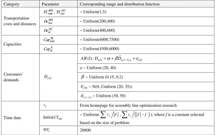
5-1-Data generation and settings
The required data for the problem instances can be characterized into four groups: transportation costs and distances, two types of maximum capacities, customers’ demands and time data. The sources of random generation and fixed values of parameters used in the problem instances are listed in Table 3.The data for ALB, i.e. task times and precedence constraints, are obtained from homepage for assembly line optimization research (www.assembly-line-balancing.de).Afterward, using the generated parameters, 15 problem instances with different sizes are constructed.
104
Table 3.Parameters values used in the problem instances
Category Parameter Corresponding range and distribution function
Transportation costs and distances
MA mat
TC , TCactAC ~ Uniform(1,5) MA
ma
Dc ~ Uniform(200,400)
AC ac
Dc ~ Uniform(400,600)
Capacities
M mkt
Cap ~ Uniform(6000,7500)
A at
Cap ~ Uniform(4500,6000)
Customers’
demands Dcts
c, 1,
ˆ
(1) : cts t s cts
AR D = +α βD − +ε
α ~ Uniform (20, 40)
β ~ Uniform (0.15, 0.2)
cts
ε ~ N(0, Uniform (20, 35))
c, 1,
ˆ t s
D − ~ Uniform (30, 50)
Time data
i
t From homepage for assembly line optimization research
InitialCTats ~ Uniform(
∑
ti J ,∑
ti(
J −f)
), where f is a constant selectedbased on the size of problem
t
WT 28800
5-2- Problem instances generation
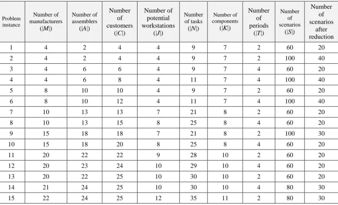
Several problem instances are randomly generated considering assumptions that reflect the real-world situation. Sizes of these problem instances are chosen based on the range of test problems presented in the literature (see for example Pishvaee et al.,( 2010)).Table 4 reports the characteristics of 15 problem instances used in this section. The size of a problem instance is determined by
105
Table 4. The characteristics of the problems instances.
5-3- Computational results
This subsection presents iteration number in which the iterative process stops, the best lower and upper objective values and the CPU time for the pre-defined problems instances. It should be noted that the stopping criterion is based on step 5 of solution method presented in section 0.The proposed solution method was coded in MATLAB 7.1 where the lower-level and upper-level models were formulated in GAMS 23.5.All experiments were run with an Intel Pentium IV dual core 2.1 GHz CPU PC at 3 GB RAM under a Microsoft Windows 7 environment.
All problem instances were solved using the proposed heuristics solution algorithm. The results for each problem instance are reported in Table 5. In addition, Figure 10 shows the convergence of the upper-level and lower-level models’ objective values (ZU and ZL) for problem instances 4, 9, 11 and
13 until the stopping criteria is met. The obtained results show that the proposed solution algorithm is efficient in solving the developed model and so this algorithm can be employed in finding the optimal solutions of problem instances with different sizes in reasonable computational time.
Problem instance
Number of manufacturers
(|M|)
Number of assemblers
(|A|)
Number of customers
(|C|)
Number of potential workstations
(|J|)
Number of tasks
(|N|)
Number of components
(|K|)
Number of periods
(|T|)
Number of scenarios
(|S|)
Number of scenarios
after reduction
1 4 2 4 4 9 7 2 60 20
2 4 2 4 4 9 7 2 100 40
3 4 6 6 4 9 7 4 60 20
4 4 6 8 4 11 7 4 100 40
5 8 10 10 4 9 7 2 60 20
6 8 10 12 4 11 7 4 100 40
7 10 13 13 7 21 8 2 60 20
8 10 13 15 8 25 8 4 60 20
9 15 18 18 7 21 8 2 100 30
10 15 18 20 8 25 8 4 60 20
11 20 22 22 9 28 10 2 60 20
12 20 23 24 10 29 10 4 60 20
13 20 22 25 10 30 10 2 60 20
14 21 24 25 10 30 10 4 80 30
106
Table 5.Theobtained results fromthe proposed solution method for the defined problems instances
Problem instance 4
Problem instance9
47.4 47.6 47.8 48 48.2 48.4 48.6 48.8 49 49.2
1 2 3 4 5 6 7 8 9 10 11 12
ZL
Iteration No.
2744920 2744940 2744960 2744980 2745000 2745020 2745040
1 2 3 4 5 6 7 8 9 10 11 12
ZU
Iteration No.
73.5 74 74.5 75 75.5 76
1 2 3 4 5 6 7 8
ZL
Iteration No.
3350700 3350720 3350740 3350760 3350780 3350800 3350820 3350840 3350860 3350880 3350900
1 2 3 4 5 6 7 8
ZU
Iteration No.
Problem instance Iteration number (to stop the
iterative process) ZU ZL CPU time
1 6 1169178 12.67 26 s
2 5 1007695 13.1 96 s
3 9 2979740 72.3 2245 s
4 12 2744954 48 3975 s
5 6 1614678 61.07 965 s
6 7 5031525 90.78 7124 s
7 10 2513249 90.28 3981 s
8 9 5902075 100.65 3788 s
9 8 3350761 74.26 8584 s
10 7 5240030 145.72 8419 s
11 10 3952291 75.57 > 3 hours
12 17 8609533 114.57 > 3 hours
13 11 4553853 75.73 7539 s
14 21 8370290 196 > 3 hours
107
Problem instance 11
Problem instance 13
Figure 10.The convergence of ZL and ZU for several problem instances 5-4- Comparison between stochastic and deterministic models
In this subsection, the performance comparison between the developed stochastic model and its equivalent deterministic version is made. In the deterministic model, the scenario indices and the corresponding probabilities (Prts) are removed from the model. In addition due to meaningful
comparison between deterministic and stochastic models, in the deterministic model, one of the generated scenarios is selected randomly for cycle time, i.e. CTats, and customer demand (Dcts) at each
period. For this purpose, several problem instances with different sizes are selected from Table 4. Figure 11and Figure 12 demonstrate the performance of the stochastic and deterministic models in terms of ZL and ZU for several problem instances defined in Subsection 0. As Figure 11 shows, the
deterministic model has obtained better ZL in all problem instances. On the other hand, Figure
12illustrates that the stochastic model obtains better ZU in comparison with deterministic model in
most of problem instances. To conclude, the developed stochastic model mainly performs better than the equivalent deterministic model in making strategic decisions while the deterministic model works better in making tactical decisions, i.e. ALB decisions.
70 75 80 85 90 95 100 105 110
1 2 3 4 5 6 7 8 9 10
ZL
Iteration No.
3000000 3500000 4000000 4500000 5000000 5500000
1 2 3 4 5 6 7 8 9 10
ZU
Iteration No.
70 75 80 85 90 95
1 2 3 4 5 6 7 8 9 10 11
ZL
Iteration No.
4553000 4553500 4554000 4554500 4555000 4555500 4556000
1 2 3 4 5 6 7 8 9 10 11
ZU
108
Figure 11. Comparison betweenstochastic and deterministic models in terms of ZL for several problem instances
Figure 12. Comparison between stochastic and deterministic models in terms of ZUfor several problem instances
6- Conclusions and future research
This paper addresses an important issue concerning the integration of strategic and tactical decisions in supply chain management. The main objective of this paper is to introduce and characterize the problem of integrating supply chain network design and assembly line balancing problems under demand uncertainty. A special case of supply chain networks is considered in which assembly activities are a main stage of the supply chain in the uncertain environment. A novel bi-level stochastic programming model is developed to design and optimize the considered supply chain including manufacturers, assemblers and customers. In order to deal with demand uncertainty, a three-step algorithm is proposed to generate different demand scenarios. Moreover, a heuristic method is proposed to solve the developed model. Finally, computational experiments over several problem instances show that the developed model is valid and capable to be employed in practical cases. The comparison between the stochastic and equivalent deterministic model is also made.
Future research can investigate multiple products, U-shaped or two-sided assembly lines and equipment selection. Considering location, routing or inventory decisions in supply chain network
1 3 5 7 10 13
Deterministic 11 72 60 88 145 74
Stochastic 12.75 72.30 61.87 90.35 146.77 75.73
0 20 40 60 80 100 120 140 160
ZL
Problem Instance #
1 3 5 7 10 13 Deterministic 1148380 2964340 1604290 2511140 5226440 4447801 Stochastic 1069339 2950740 1606181 2474083 5216087 4441279
0 1000000 2000000 3000000 4000000 5000000 6000000
ZU
109
design problem is also a valuable future work. In addition, since CPU time increases significantly when problem size and the number of scenarios increase, developing meta-heuristic algorithms or exact solution methods (such as branch-and-bound method) to solve large-scale problems is of interest for future studies.
References
Arzu Akyuz, G., & Erman Erkan, T. (2010). Supply chain performance measurement: a literature review. International Journal of Production Research, 48(17), 5137-5155.
Babazadeh, R., Razmi, J., & Ghodsi, R. (2012). Supply chain network design problem for a new market opportunity in an agile manufacturing system. Journal of Industrial Engineering International, 8(1), 19.
Becker, C., & Scholl, A. (2006). A survey on problems and methods in generalized assembly line balancing. European journal of operational research, 168(3), 694-715.
Ben-Ayed, O., Boyce, D. E., & Blair, C. E. (1988). A general bilevel linear programming formulation of the network design problem. Transportation Research Part B: Methodological, 22(4), 311-318.
Bidhandi, H. M., & Yusuff, R. M. (2011). Integrated supply chain planning under uncertainty using an improved stochastic approach. Applied Mathematical Modelling, 35(6), 2618-2630.
Birge, J. R., & Louveaux, F. (2011). Introduction to stochastic programming. Springer Science & Business Media.
Cardona-Valdés, Y., Álvarez, A., & Ozdemir, D. (2011). A bi-objective supply chain design problem with uncertainty. Transportation Research Part C: Emerging Technologies, 19(5), 821-832.
Carle, M. A., Martel, A., & Zufferey, N. (2012). The CAT metaheuristic for the solution of multi-period activity-based supply chain network design problems. International Journal of Production Economics, 139(2), 664-677.
Chen, T. L., & Lu, H. C. (2012). Stochastic multi-site capacity planning of TFT-LCD manufacturing using expected shadow-price based decomposition. Applied Mathematical Modelling, 36(12), 5901-5919.
Chopra, S., & Meindl, P. (2007). Supply chain management. Strategy, planning & operation. Das summa summarum des management, 265-275.
Colson, B., Marcotte, P., & Savard, G. (2005). Bilevel programming: A survey. 4OR: A Quarterly Journal of Operations Research, 3(2), 87-107.
Costa, A., Celano, G., Fichera, S., & Trovato, E. (2010). A new efficient encoding/decoding procedure for the design of a supply chain network with genetic algorithms. Computers & Industrial Engineering, 59(4), 986-999.
Dupačová, J., Gröwe-Kuska, N., & Römisch, W. (2003). Scenario reduction in stochastic programming. Mathematical programming, 95(3), 493-511.
Georgiadis, M. C., Tsiakis, P., Longinidis, P., & Sofioglou, M. K. (2011). Optimal design of supply chain networks under uncertain transient demand variations. Omega, 39(3), 254-272.
Ghiani, G., Laporte, G., & Musmanno, R. (2004). Introduction to logistics systems planning and control. John Wiley & Sons.
110
Hamta, N., Shirazi, M. A., & Ghomi, S. F. (2016). A bi-level programming model for supply chain network optimization with assembly line balancing and push–pull strategy. Proceedings of the Institution of Mechanical Engineers, Part B: Journal of Engineering Manufacture, 230(6), 1127-1143.
Hamta, N., Akbarpour Shirazi, M., Fatemi Ghomi, S. M. T., & Behdad, S. (2015). Supply chain network optimization considering assembly line balancing and demand uncertainty. International Journal of Production Research, 53(10), 2970-2994.
Hamta, N., Ghomi, S. F., Jolai, F., & Shirazi, M. A. (2013). A hybrid PSO algorithm for a multi-objective assembly line balancing problem with flexible operation times, sequence-dependent setup times and learning effect. International Journal of Production Economics, 141(1), 99-111.
Hamta, N., Ghomi, S. F., Jolai, F., & Bahalke, U. (2011). Bi-criteria assembly line balancing by considering flexible operation times. Applied Mathematical Modelling, 35(12), 5592-5608.
Iman, R. L. (2008). Latin hypercube sampling. John Wiley & Sons, Ltd.
Javid, A. A., & Azad, N. (2010). Incorporating location, routing and inventory decisions in supply chain network design. Transportation Research Part E: Logistics and Transportation Review, 46(5), 582-597.
Khalili-Damghani, K., Tavana, M., & Amirkhan, M. (2014). A fuzzy bi-objective mixed-integer programming method for solving supply chain network design problems under ambiguous and vague conditions. The International Journal of Advanced Manufacturing Technology, 73(9-12), 1567-1595.
Klibi, W., Martel, A., & Guitouni, A. (2010). The design of robust value-creating supply chain networks: a critical review. European Journal of Operational Research, 203(2), 283-293.
Kristianto, Y., Gunasekaran, A., Helo, P., & Hao, Y. (2014). A model of resilient supply chain network design: A two-stage programming with fuzzy shortest path. Expert Systems with Applications, 41(1), 39-49.
Lin, C. C., & Wang, T. H. (2011). Build-to-order supply chain network design under supply and demand uncertainties. Transportation Research Part B: Methodological, 45(8), 1162-1176.
Longinidis, P., & Georgiadis, M. C. (2011). Integration of financial statement analysis in the optimal design of supply chain networks under demand uncertainty. International journal of production economics, 129(2), 262-276.
Martínez-Jurado, P. J., & Moyano-Fuentes, J. (2014). Lean management, supply chain management and sustainability: a literature review. Journal of Cleaner Production, 85, 134-150.
Melo, M. T., Nickel, S., & Saldanha-Da-Gama, F. (2009). Facility location and supply chain management–A review. European journal of operational research, 196(2), 401-412.
Melo, M. T., Nickel, S., & Saldanha-da-Gama, F. (2012). A tabu search heuristic for redesigning a multi-echelon supply chain network over a planning horizon. International Journal of Production Economics, 136(1), 218-230.
Nickel, S., Saldanha-da-Gama, F., & Ziegler, H. P. (2012). A multi-stage stochastic supply network design problem with financial decisions and risk management. Omega, 40(5), 511-524.
111
Olsson, A., Sandberg, G., & Dahlblom, O. (2003). On Latin hypercube sampling for structural reliability analysis. Structural safety, 25(1), 47-68.
Paksoy, T., & Özceylan, E. (2012 a). Supply chain optimisation with U-type assembly line balancing. International Journal of Production Research, 50(18), 5085-5105.
Paksoy, T., Özceylan, E., & Gökçen, H. (2012 b). Supply chain optimisation with assembly line balancing. International Journal of Production Research, 50(11), 3115-3136.
Paksoy, T., Pehlivan, N. Y., & Özceylan, E. (2012 c). Application of fuzzy optimization to a supply chain network design: a case study of an edible vegetable oils manufacturer. Applied Mathematical Modelling, 36(6), 2762-2776.
Pishvaee, M. S., Farahani, R. Z., & Dullaert, W. (2010). A memetic algorithm for bi-objective integrated forward/reverse logistics network design. Computers & operations research, 37(6), 1100-1112.
Pishvaee, M. S., Jolai, F., & Razmi, J. (2009). A stochastic optimization model for integrated forward / reverse logistics network design. Journal of Manufacturing Systems, 28(4), 107-114.
Roni, M. S., Eksioglu, S. D., Searcy, E., & Jha, K. (2014). A supply chain network design model for biomass co-firing in coal-fired power plants. Transportation Research Part E: Logistics and Transportation Review, 61, 115-134.
Rezapour, S., Farahani, R. Z., Ghodsipour, S. H., & Abdollahzadeh, S. (2011). Strategic design of competing supply chain networks with foresight. Advances in Engineering Software, 42(4), 130-141.
Sadjady, H., & Davoudpour, H. (2012). Two-echelon, multi-commodity supply chain network design with mode selection, lead-times and inventory costs. Computers & Operations Research, 39(7), 1345-1354.
Santoso, T., Ahmed, S., Goetschalckx, M., & Shapiro, A. (2005). A stochastic programming approach for supply chain network design under uncertainty. European Journal of Operational Research, 167(1), 96-115.
Shen, Z. (2007). Integrated supply chain design models: a survey and future research directions. Journal of Industrial and Management Optimization, 3(1), 1.
Schmidt, G., & Wilhelm, W. E. (2000). Strategic, tactical and operational decisions in multi-national logistics networks: a review and discussion of modelling issues. International Journal of Production Research, 38(7), 1501-1523.
Schütz, P., Tomasgard, A., & Ahmed, S. (2009). Supply chain design under uncertainty using sample average approximation and dual decomposition. European Journal of Operational Research, 199(2), 409-419.
Simchi-Levi, D., Kaminsky, P., & Simchi-Levi, E. (2004). Managing The Supply Chain: Definitive Guide. Tata McGraw-Hill Education.
Singh, A. R., Jain, R., & Mishra, P. K. (2013). Capacities-based supply chain network design considering demand uncertainty using two-stage stochastic programming. The International Journal of Advanced Manufacturing Technology, 69(1-4), 555-562.
Sun, H., Gao, Z., & Wu, J. (2008). A bi-level programming model and solution algorithm for the location of logistics distribution centers. Applied mathematical modelling, 32(4), 610-616.
112
Sung, C. S., & Song, S. H. (2003). Integrated service network design for a cross-docking supply chain network. Journal of the Operational Research Society, 54(12), 1283-1295.
Tsao, Y. C., & Lu, J. C. (2012). A supply chain network design considering transportation cost discounts. Transportation Research Part E: Logistics and Transportation Review, 48(2), 401-414.
Tsiakis, P., & Papageorgiou, L. G. (2008). Optimal production allocation and distribution supply chain networks. International Journal of Production Economics, 111(2), 468-483.
Vahdani, B., Tavakkoli-Moghaddam, R., Jolai, F., & Baboli, A. (2013). Reliable design of a closed loop supply chain network under uncertainty: An interval fuzzy possibilistic chance-constrained model. Engineering Optimization, 45(6), 745-765.
Vidal, C. J., & Goetschalckx, M. (1997). Strategic production-distribution models: A critical review with emphasis on global supply chain models. European journal of operational research, 98(1), 1-18. Wang, F., Lai, X., & Shi, N. (2011). A multi-objective optimization for green supply chain network design. Decision Support Systems, 51(2), 262-269.
Werner, A. (2005). Bilevel stochastic programming problems: Analysis and application to telecommunications.