The Existence of Noise Terms for Systems of Partial Differential and Integral Equations with (HPM) Method

(1)

The Existence of Noise Terms for Systems of Partial

Differential and Integral Equations with ( HPM ) Method

Parivash Shams Derakhsh

*

_{, Jafar Biazar}

Department of Mathematics, Faculty of Science University of Guilan *Corresponding Author: [email protected]

Abstract

In this paper we develop a framework for necessary condition for the existence of noise terms for systems of partial differential and integral equations with ( HPM ) method. We show that the noise terms are conditional and are generated for inhomogeneous equations if specific criteria is justified. And to illustrate the capability and reliability of this method We numerically test our approach for a variety of systems of inhomogeneous problems.

Keywords

Partial Differential, Integral Equations, Homotopy Perturbation Method, Phenomenon

MSC(2010)No: 34A34; 31A10

1. Introduction

Homotopy perturbation method ( HPM ) is useful and powerful method for solving linear and nonlinear differential equations. A brief discussion of Homotopy perturbation method will be emphasized, the complete details of the method are found in [3-5]. The Homotopy perturbation method goal is to find the solution of linear and nonlinear, partial differential equations and integral equations with dependence on small parameter. In this method the solution is considered as sum of an infinite series which, rapidly convergence to an accurate solutions. Systems of partial differential equations and integral equations were formally derived to describe nonlinear waves and arise in gas dynamics, water waves [6-10], flood waves in rivers, traffic flow and a wide range of biological and ecological systems. The noise terms phenomenon [11-15] gives a useful tool in that, if it appears, it gives a fast convergence of the solution by using two iterations only. It is important to note that these terms may appear for inhomogeneous problems, whereas homogeneous problems do not generate noise terms. It was formally shown that by canceling the noise terms that appear

u0 and u1 from u0, even though u1 contains further terms, the remaining noncancelled terms of u0 may give the exact solution of the inhomogeneous problem. A complete and thorough study on noise terms can be found in details in [11-15].

2. The Noise Terms Phenomenon

The noise terms phenomenon [8–12] gives a useful tool in that, if it appears,it gives a fast convergence of the solution by using two iterations only.

It is significant to note that the noise terms may appear only for inhomogeneous problems.

The noise terms are defined as the identical terms, with opposite signs, that may appear in various components uk , k ≥1. It is important to note that these terms may appear for inhomogeneous problems, whereas homogeneous problems do not generate noise terms. It was formally shown that by canceling the noise terms that appear in u0 and u1 from u0, even though u1 contains further terms, the remaining noncancelled terms of u0 may give the exact solution of the inhomogeneous problem. This can be justified through substitution. Therefore, it is necessary to verify that the noncancelled terms of u0 satisfy the PDE under discussion. A necessary condition for the generation of the noise terms for inhomogeneous problems is that the zeroth component u0 must contain the exact solution u among other terms. A complete and thorough study on noise terms can be found in details in [8–12]. To give a clear overview of the content of this work, several illustrative examples of systems of partial differential and integral equations, have been selected to demonstrate the efficiency of the method and to confirm the necessary condition needed for the generation of the noise terms.

(2)

(1) With initial data

(2) Where N1, N2,…Nn are nonlinear operators and g1,g2,..gn are inhomogeneous terms. To solve system (1) by homotopy perturbation method, we construct the following homotopies:

(3) Consider the solution of the system (3) as the following

U1 = U10 + p U11+p2_{U12 +…,}

U2 = U20 + P U21+p2_{U22 +…. (4)} Equating the coefficients of the terms with the identical powers of p leads to

(3)

So we have

U11(x,t) = - ∫(𝜕𝜕𝑈𝑈20 𝜕𝜕𝑥𝑥1 𝑡𝑡

0 +⋯+

𝜕𝜕𝑈𝑈𝑛𝑛0

𝜕𝜕𝑥𝑥𝑛𝑛 −1 +M 10 -g1) dt,

U11(x,t) = - ∫(𝜕𝜕𝑈𝑈10_{𝜕𝜕𝑥𝑥}

1 𝑡𝑡

0 +⋯+

𝜕𝜕𝑈𝑈𝑛𝑛0

𝜕𝜕𝑥𝑥𝑛𝑛 −1 +M 20 -g2) dt, ⋮

Un1(x,t) = - ∫(𝜕𝜕𝑈𝑈20_{𝜕𝜕𝑥𝑥}

1 𝑡𝑡

0 +⋯+

𝜕𝜕𝑈𝑈10

𝜕𝜕𝑥𝑥𝑛𝑛 −1 +Mn0-gn) dt,

For j>1, we derive

Unj(x,t) = - ∫(𝜕𝜕𝑈𝑈2𝑗𝑗−1 𝜕𝜕𝑥𝑥1 𝑡𝑡

0 +⋯+

𝜕𝜕𝑈𝑈𝑖𝑖𝑗𝑗 −1

𝜕𝜕𝑥𝑥𝑛𝑛 −1 +Mnj-1) dt,

The approximate solutions of (1) can be obtained by letting p tend to one

4. Numerical Example

4.1. Systems of Integral Equations

In what follows we will examine the noise terms phenomenon by studying a system of inhomogeneous integral equations.

Example1. We first consider the inhomogeneous systems: u(x) = 1+∫ 𝑢𝑢𝑥𝑥 2

0 v dx, (4) v(x) = 1-∫ 𝑣𝑣𝑥𝑥 2

0 u dx (5)

Suppose the solution of Eq.(4) and Eq.(5) has the following form

U= U0 + pU1+ p2_{U2 +….. (6)} V= V0 + pV1+ p2_{V2 +….. (7)} Using the series (4) and (5) for the linear terms u(x) and v(x) and for the nonlinear terms u2_{v and v}2_{u, and by Substituting} Eq.(6) and Eq.(7) into Eq.(4) and Eq.(5) and equating the terms with identical powers of p leads to

（8）

Successive solution of Eq.(8) yields to ( U0(x), V0(x) ) = (1,1), ( U1(x), V1(x) ) = (x,-x), ( U2(x) , V2(x) ) = ( 𝑥𝑥₂2,−𝑥𝑥₂2),

⋮

Combining these results yields the series solutions U(x) = 1+ x + 𝑥𝑥₂2 + 𝑥𝑥₆3 +…. ,

V(x) = 1- x + 𝑥𝑥₂2 - 𝑥𝑥₆3 +…. . So that the solutions in closed forms are given by

U(x) = 𝑒𝑒𝑥𝑥_,

V(x) = 𝑒𝑒−𝑥𝑥_.

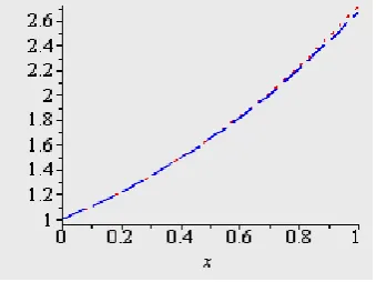
[image:3.595.62.275.91.216.2]

An important remark can be made here in that although the problem is an inhomogeneous problem, the noise terms did not appear between various component.

Figure 1. Graph of uexact ,uHPM for example 1

Figure 2. Graph of vexact ,vHPM for example1

Example 2. We next consider the inhomogeneous systems: u(x,t) = x +𝑒𝑒𝑥𝑥−𝑡𝑡_-_{∫ 𝑢𝑢𝑣𝑣}𝑥𝑥

[image:3.595.348.518.412.539.2]

(4)

v(x,t) = -x+𝑒𝑒−𝑥𝑥+𝑡𝑡₊_{∫ 𝑢𝑢}𝑥𝑥 2_𝑣𝑣2

0 dx.

By using homotopy perturbation method we have

(9) Successive solution of Eq.(9) yields to

( U0(x,t) ,V0(x,t) ) = ( x+ 𝑒𝑒𝑥𝑥−𝑡𝑡_{, -x+}_𝑒𝑒−𝑥𝑥+𝑡𝑡_),

( U1(x,t),V1(x,t) ) = (-x+ 1₃ 𝑥𝑥3_{+ exponential terms , x+}1

5 𝑥𝑥5+ exponential terms ),

⋮

We can easily observe the noise terms ± x in the components U0 and U1, and the noise terms ∓x in the component V0 and V1. By canceling these terms from U0 and V0 and by justifying that the remaining terms in the zeroth components justify the inhomogeneous problems , we have:

U(x,t) = 𝑒𝑒𝑥𝑥−𝑡𝑡_,

V(x,t) = 𝑒𝑒−𝑥𝑥+𝑡𝑡_.

[image:4.595.58.292.100.408.2]

Other noise terms between other component vanish in the limit.

Figure 3. Graph of example 2; Uexact (x,0.02)

….

, UHPM (x,0.03) __ __;

[image:4.595.347.520.121.247.2]

UHPM(x,0.02)

- - - -

,UHPM (x,0.04) ____

Figure 4. Graph of example 2; Vexact (x,0.02)

….

,VHPM (x,0.04) __ __; VHPM (x,0.02)

- - - -

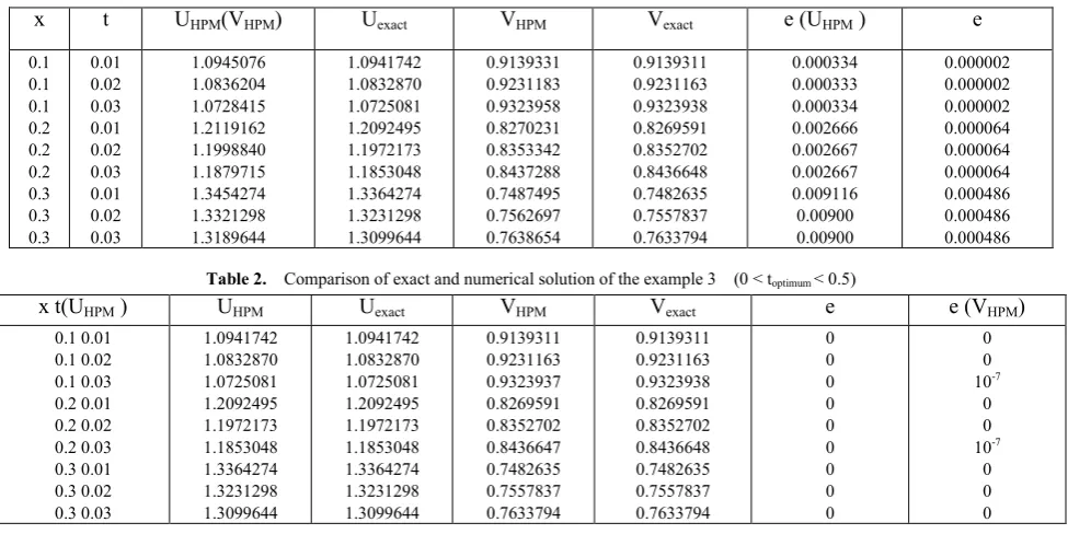
, VHPM (x,0.03) ____

Table 1. Comparison of exact and numerical solution of the example 2 (0 < toptimum < 0.5)

x t UHPM(VHPM) Uexact VHPM Vexact e (UHPM ) e

0.1 0.1 0.1 0.2 0.2 0.2 0.3 0.3 0.3 0.01 0.02 0.03 0.01 0.02 0.03 0.01 0.02 0.03 1.0945076 1.0836204 1.0728415 1.2119162 1.1998840 1.1879715 1.3454274 1.3321298 1.3189644 1.0941742 1.0832870 1.0725081 1.2092495 1.1972173 1.1853048 1.3364274 1.3231298 1.3099644 0.9139331 0.9231183 0.9323958 0.8270231 0.8353342 0.8437288 0.7487495 0.7562697 0.7638654 0.9139311 0.9231163 0.9323938 0.8269591 0.8352702 0.8436648 0.7482635 0.7557837 0.7633794 0.000334 0.000333 0.000334 0.002666 0.002667 0.002667 0.009116 0.00900 0.00900 0.000002 0.000002 0.000002 0.000064 0.000064 0.000064 0.000486 0.000486 0.000486

Table 2. Comparison of exact and numerical solution of the example 3 (0 < toptimum < 0.5)

x t(UHPM ) UHPM Uexact VHPM Vexact e e (VHPM)

[image:4.595.343.521.279.409.2] [image:4.595.62.550.513.757.2]

(5)

4.2. System of Partial Differential Equations

Example 3.consider the system of inhomogeneous partial differential equations

With the initial data

u(x,0) =𝑒𝑒𝑥𝑥_,

v(x,0) = 𝑒𝑒−𝑥𝑥_.

By using Eq.(6) and Eq.(7) for the linear terms u(x,y) and v(x,y) we have

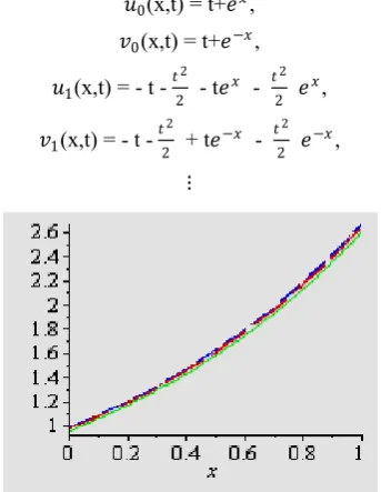
𝑢𝑢0(x,t) = t+𝑒𝑒𝑥𝑥,

𝑣𝑣0(x,t) = t+𝑒𝑒−𝑥𝑥,

𝑢𝑢1(x,t) = - t -𝑡𝑡

2

2 - t𝑒𝑒𝑥𝑥 -

𝑡𝑡2

2 𝑒𝑒𝑥𝑥,

𝑣𝑣1(x,t) = - t -𝑡𝑡

2

2 + t𝑒𝑒−𝑥𝑥 -

𝑡𝑡2

2 𝑒𝑒−𝑥𝑥,

[image:5.595.92.264.267.489.2]

⋮

Figure 5. Graph of example 3; Uexact (x,0.02) - - - ,UHPM (x,0.02) ...; UHPM

(x,0.03) __ __,UHPM(x,0.04) ___

Figure 6. Graph of example 3; Vexact (x,0.02) - - - - ,VHPM (x,0.02) ……;

VHPM (x,0.03) __ __ ,VHPM (x,0.04) ____

We see that the terms ± t in 𝑢𝑢0 and 𝑢𝑢1 cannot be considered noise terms that will lead to the exact solution. this can be attributed to the fact that by canceling that term from u0 will give u0 =𝑒𝑒𝑥𝑥_{wich is not the exact solution.}

Accordingly, the solution in a series form is given by

( U,V ) = (𝑒𝑒𝑥𝑥_{(1- t +}𝑡𝑡2

2

-𝑡𝑡3

6 +…) ,𝑒𝑒−𝑥𝑥(1+ t +

𝑡𝑡2

2 +

𝑡𝑡3

6 +…)),

and in a closed form we have

( U,V ) = (𝑒𝑒𝑥𝑥−𝑡𝑡_,_𝑒𝑒−𝑥𝑥+𝑡𝑡_).

Since Homotopy perturbation method hase been led to the exact solution comparison in examples of the results in figs and tables are informative any more.

4. Conclusions

In this article, we have applied homotopy perturbation method for solving noise terms in partial differential and integral equations. The approximate solutions obtained by Homotopy perturbation method are compared with the exact solutions. The results show that the Homotopy perturbation method is powerful mathematical tool for solving systems of nonlinear partial differential equations, which appears in mathematical modeling of different phenomena. This model has been solved by Adomian method,as well [16]. Homotopy perturbation method in comparison with Adomian,_{s decomposition method has the}

advantage of overcoming the difficult arising in calculating Adomian polynomials . From tables we see that errors are very low, and near the exact solutions. The computations associated with the examples in this work were performed using maple13.

REFERENCES

[1] G. Adomian, A review of the decomposition method in applied mathematics, J. Math. Anal. Appl. 135 (1988) 501_544.

[2] G. Adomian, Solving Frontier Problems of Physics: The Decomposition Method, Kluwer Academic Publishers, Boston, 1994.

[3] Ariel, P.D., Hayat, T., Asghar, S., 2006. Homotopy perturbation method and axisymmetric flow over a stretching sheet. International Journal of Nonlinear Science and Numerical Simulation 7(4), 399–406.

[4] Biazar, J., Eslami, M., Ghazvini, H., 2007. Homotopy perturbation method for systems of partial differential equations. International Journal of Nonlinear Science and Numerical Simulation 8 (3), 411–416.

[5] Kythe, P.K. and P. Puri, 2002. Computational methods for linear integral equations. University of New Orlans, New Orlans.

[6] L. Debnath, Nonlinear Partial Differential Equations for Scientists and Engineers,Birkhauser, Boston, 1997.

[7] J.D. Logan, An Introduction to Nonlinear Partial Differential Equations, Wiley-Interscience,New York, 1994.

(6)

York, 1974.

[9] C. Lubich, A. Ostermann, Multigrid dynamic interaction for parabolic equations, BIT 27 (1987) 216–234.

[10] S. Vandewalle, R. Piessens, Numerical experiments with nonlinear multigrid waveformrelaxation on a parallel processor, Appl. Numer. Math. 8 (1991) 149–161.

[11] A.M.Wazwaz, Partial Differential Equations: Methods and Applications, Balkema Publishers, Lisse, the Netherlands, 2002.

[12] A.M. Wazwaz, A First Course in Integral Equations, WSPC, New Jersey, 1997.

[13] A.M. Wazwaz, Exact solutions to nonlinear diffusion equations by the decomposition method,Appl. Math. Compute. 123 (1) (2001) 109–122.

[14] A.M. Wazwaz, Analytical approximations and Pade_ approximants for Volterras population model, Appl. Math. Compute. 100 (1999) 13–25.

[15] A.M. Wazwaz, Necessary conditions for the appearance of noise terms in decomposition solution series, Appl. Math. Compute. 81 (1997) 139–147.