Mapping and Simulating Watershed Performances
Based on GIS, Remote Sensing, and SWAT
Sandhyavitri Ari
1, Yusa Muhamad
1,*, Fajri Mardan
1, Sutikno Sigit
1, Arai Kohei
21Civil Engineering Department, University of Riau, Pekanbaru, 28293, Indonesia 2Department of Information Science, Saga University, Saga, Japan
Copyright©2018 by authors, all rights reserved. Authors agree that this article remains permanently open access under the terms of the Creative Commons Attribution License 4.0 International License
Abstract
This study has demonstrated that the combination of the geographic information systems (GIS), remote sensing (RS), and the Soil and Water Assessment Tool (SWAT) has yield a comprehensive land use mapping and an assessment report of watershed performances. The Tapung watershed located in sub-watershed of Siak, Riau Province, Indonesia was appointed as a study area. This research identified that the existing land use condition (in 2012) was dominated by oil palm plantation (46%), agriculture (24%), and bushes including shrubs (8%), and a small number of forest area (7%). Thus, there was a need for conducting reforestation management programs within the watershed areas in order to maintain the watershed performances. However, based on this study the existing watershed performances (scenario 1) was in the state of moderate conditions as the percentage of the critical coverage areas (PLK) was small (10.41%), with the annual water flow coefficient or water run-off (KRA) was high (0.45). Hence, there was a need to reduce this run-off to become <30% by conducting the watershed management programs. This study also simulated the future of the watershed performances using the Soil and Water Assessment Tool (SWAT). After conducting the conservation programs (scenario 2), it was revealed that the watershed indicators performance would be improved. The results model of this watershed is also considered acceptable as the determination coefficient (R2) = 0.50 > 0.40 and NS = 0.50 > 0.36. Hence, this study confirmed that the GIS, RS, and SWAT were capable for mapping and simulating the watershed performances systematically.Keywords
Geographic Information Systems (GIS), Remote Sensing (RS), Watershed Performances, Land Use Change, SWAT1. Introduction
The Siak river with 50-75m in width and 672 in length, used to be the deepest river in Indonesia with 20-30 meters depth [1]. Surprisingly, its depth decreased significantly to become 8-13 meter in 2015 [1, 2] indicating there has been a serious deterioration process of its watershed health performances [3]. This fact shows that there is an urgent need to develop Tapung watershed map to understand the change in land use pattern within the watershed area. This in turn can be used to investigate watershed performances. Based on a number of watershed publications it is identified that the Soil and Water Assessment Tool (SWAT) capable in simulating watershed performances [3-7].
The land use of Tapung watershed has been shifting in a massive scale from the forest area to become palm oil plantation or to become residential, farming and agricultural areas (Figure 1). These significant changes of land use were suspected to deteriorate the watershed performances [8].
Figure 1. The location of Tapung watershed, Riau Province, Indonesia
The main objectives of this study are to; (i) develop Tapung watershed land use map located in Siak River, Indonesia using combination of the Geographic Information Systems (GIS) and remote sensing (RS) in the period of 2002, 2007, 2012, and (ii) simulate the watershed performances based on the existing government regulations for watershed condition in 2012 (scenario 1), and the future condition after an application of conservation scheme (scenario 2), then (iii) develop hydrological models of this Tapung watershed.
2.
Methodology/ Experimental
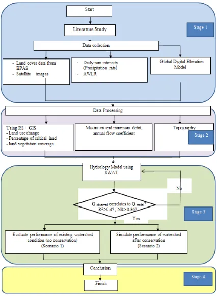
2.1. Research Flowchart
In general the methodology used in this research is shown by the following flowchart (Figure 2). There are 4 (four) major stages which was conducted in this research; (i) data collections encompassing; literature study, land cover maps data, satellite images, rain intensity, and digital elevation model data; (ii) data processing encompassing;
development of land use maps, critical land information, and vegetation classification maps; annual flows; and topography maps (however not all maps would be presented in this paper); (iii) developing hydrology models using SWAT (compromising Scenario 1 and 2); and (iv) result findings and a conclusion.
[image:2.595.62.538.77.387.2]Table 1. Evaluation Criteria for Watershed Performances [9,10].
Notes:
The percentage of critical land area areas (PLK) range standard values was as follow; PLK ≤ 5% very low, 5% <
PLK ≤ 10% low, 10% < PLK ≤ 15% moderate, 15% < PLK ≤ 20% high, and PLK > 20% very high. The lower the
PLK value the better watershed performance would be.
The percentage of vegetation coverage areas (PPV) > 80% excellent, 60% < PPV ≤ 80% good, 40% < PPV ≤ 60%
moderate, 20% < PPV ≤ 40% poor, and PPV ≤ 20% worst. The higher the PLK value the better watershed
performance would be.
The water flow regime coefficient (KRA) ≤ 20 very low, 20 < KRA ≤ 50 low, 50 < KRA ≤ 80 moderate, 80 <
KRA ≤ 110 high, and KRA > 110 very high. The lower the PLK value the better watershed performance would be.
The annual water flow coefficient (KAT) ≤ 0.2 very low, 0.2 < KAT ≤ 0.3 low, 0.3 < KAT ≤ 0.4 moderate, 0.4 <
KAT ≤ 0.5 high, and KAT > 0.5 very high. The lower the PLK value the better watershed performance would be.
2.2. Location and Data Sources
The location of this study is in Tapung watershed, Riau, Indonesia (Figures 1 and 3). The data used in this study were; ground water level, climatic data, land use and RS images. The ground water level data were analyzed from the year 2001 to 2012. The data was obtained from the automatic water level record (AWLR) station, located in Pantai Cermin village, Kampar District, Riau with the geographical location of 00 ° 35 '24 "latitude and 101 ° 11' 46" East (Figure 1 and 3).
Figure 3. The location of the automatic water level record (AWLR) station at Pantai Cermin, sub-Siak Watershed, Riau Province, Indonesia
[image:4.595.86.509.468.733.2]The climatic data including precipitation was obtained from http://globalweather.tamu.edu/. The existing land cover data was obtained from the Watershed Management Board [11]. The RS images data were obtained from the NOAA satellite of Landsat ETM+ (Enhanced Thematic Mapper) with 30 m spatial resolution for 2002, 2007 and 2012 images. The topographic data was taken from the ASTER GDEM (Global Digital Elevation Model) with a resolution of 30 m. (http://gdem.ersdac.jspacesystems.or.jp/). [12]
3. Results and Discussion
3.1. Mapping of Sub-Siak Watershed Based on Remote Sensing (RS)
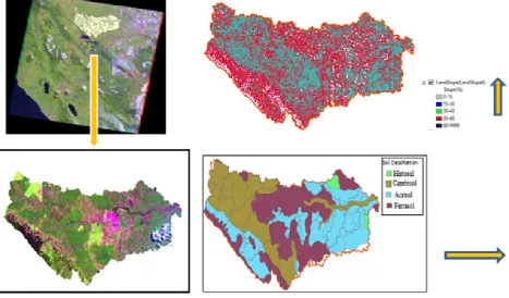
A spatial map of the sub-Siak watershed was the developed based on Geographic Information System (GIS) and Remote Sensing (RS) (Figure 4).
Figure 4. Interpretation of satellite image of Tapung watershed using GIS and RS
[image:5.595.67.535.253.527.2]Figure 5. The existing land use of the sub-Siak watershed in 2012 (Scenario 1):
[image:6.595.173.424.255.542.2]Table 2. Land use data of sub-Siak watershed, in 2012
Figure 6. Waru (Hibiscus tiliaceus rubra) and Kayu Ara (Ficus sp).
There are many soils, and water simulation models may asses the impacts of the different land use practices on the water watershed areas [13]. The Soil and Water Assessment Tool (SWAT) [6, 14] is used in this study because it has been used widely in the world [15]. This SWAT was used in this study to develop the Tapung watershed hydrological model in order to predict the long-term impact of land management practices on the existing watershed.
3.2. Simulation of the Watershed Performances
The simulation of Tapung watershed was conducted to develop the hydrology models of the existing watershed condition in 2012 (scenario 1), and future watershed condition after the reforestation conservation program has
been applied (scenario 2). The scenario 2 would be implemented within the scrubs and arid areas (critical land areas) (Figure 4). The watershed map was developed using GIS and utilizing remote sensing (RS) data obtained from the extraction of Landsat satellite images data, which have a spatial resolution of 30 m. Supervised classification method and image interpretation techniques were then applied in obtaining the land use map of 2012.
The following watershed indicator performances were presented as follow:
conservation scheme (Scenario 2), the scrubs and arid land areas were decreased to become 9,989 ha and 1,221 ha respectively. The percentage of the critical lands cover would decline from 10.41% to 6.47%. At the scenario 1, the PLK condition was moderate (10.41%), it means that there was a need attention to conduct conservation program for this watershed. The PLK of scenario 2 has decreased the watershed critical level from moderate to become low (6.4%). Hence, there was no special attention to manage the watershed (Table 1). This scenario 2 result was better than that the scenario 1 result.
Percentage of vegetation coverage areas (PPV). It was identified that the total vegetation coverage areas in 2012 was 121,829 ha and the total watershed area were 170,200 ha. The percentage of vegetation coverage areas was calculated based on the total vegetation area (121,829 ha) divided by the total watershed area (170,200 ha) = 71.6%. This result has identified that the overall PPV parameter was considered as good (> 60%) (Table 1). After conducting a simulating for scenario 2 by implementing conservation programs for arid and bushes area, it was revealed that the percentage of vegetation coverage areas becomes slightly better 124,286/170,200 = 73%. Based on the Minister of Forestry of the Republic of Indonesia Decree, Number: P. 61 / Menhut II / 2014, this value is classified as good watershed conditions (The Minister of Forestry of the Republic of Indonesia Decree, 2014) [9]. Hence there was no an urgent attention required to manage the watershed based on the parameter of vegetation coverage area for both scenario 1 and 2.
The water flow regime coefficient (KRA). This KRA value was obtained from the ratio of the maximum Tapung (sub Siak) river flow rate (Qmaks) divided by the minimum flow rate (Qmin) located within the watershed.
The Qmaks value of the Tapung watershed in 2012 was 191.52 m3 / sec, while the Qmin is 13.14 m3 / sec. Then the KRA value of this watershed in 2012 was 191.52 / 13.14 = 14.58 (very low). This means that the higher the KRA value the more the river within the watershed to cause flooding in the period of rainy season or drought in the dry season [16]. Hence, at the overall calculation in the period of 2002-2012 the KRA coefficient of this watershed was relatively very good as KRA < 20 (very low) except in 2003, the condition was dropped to 31 (low or good). This was because of in 2003 there was a period of long-dry season condition caused by the El-Nino effect.
The annual water flow coefficient (KAT). This parameter was obtained from the comparison between the annual river water flows (Q) with the precipitation thickness (P). The KAT are dynamic functions of various hydrology parameters including global weather conditions such as rainfall, temperature, humidity and wind speed. The annual water flow (Q) was obtained from the data observation of the discharge of water volume and it is divided by the total area of this watershed. The slower the infiltration rate, the more water run-off will be. As the
consequences of the rain water will go directly into the river flow or sea water. The KAT result was then converted into units of mm, while the value of precipitation (P) was taken from http://globalweather.tamu.edu/.
The existing of Q value of water discharge in 2012 was 1398.27 mm, and P value was 3117.64 mm. The annual flow coefficient was 0.45. This means that 45% of rain-water indirectly becomes run-off. After simulating conservation, it was identified that the water flow Q = 1390.36 and the value of P = 3117.64. Then the annual flow coefficient was 1390.35/3117.64 = 0.44 (< 0.45). This scenario 2 result was slightly better than that in the scenario 1.
3.3. The Hydrological Simulation Model Using Swat In order to yield the acceptable output of the hydrological model, the analyses have been applied in 4 stage such as; GIS processing, the configuration of input files in SWAT, model running, and last but not least conducting a reading out-put. Obviously, these stages required several iterations in order to yield optimum results complying with the output parameter standards (R2 and NS) (Table 3 and 4). These results also in need to be validated.
The statistical methods used to validate the model by calculating the coefficient of determination (R2) and the Nash - Sutcliffe efficiency model (NS) as presented in equations of (1) and (2).
(1)
(2) Which are:
Qobs = rate of flow observation (m3/second),
Qcal = simulated rate of flow obtained from the SWAT (m3/second),
Ǭobs = an average rate of flow observation (m3/second),
Ǭcal = an average simulated rate of flow obtained from the SWAT (m3/second).
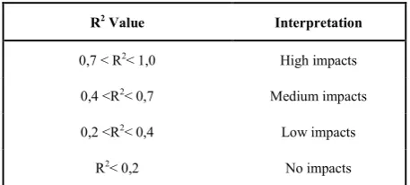
[image:7.595.307.536.629.732.2]The determination coefficient criteria (R2) were defined as the following table.
Table 3. Criteria of Determination coefficient
R2 Value Interpretation
0,7 < R2< 1,0 High impacts
0,4 <R2< 0,7 Medium impacts
0,2 <R2< 0,4 Low impacts
R2< 0,2 No impacts
Hambali, 2008 [16] suggested 4 criteria of determination coefficient. This started from R2< 0,2 (no impacts) and up to 0,7 < R2< 1,0 (high impacts).
[image:8.595.60.291.172.255.2]Motovilov, Y.G., Gottschalk, L., Engeland, K. & Rodhe, A. 1999 [17], recommended Nash-Sutcliffe Efficiency (NSE) as the following table.
Table 4. Nash-Sutcliffe Efficiency (NSE) criteria
NSE Interpretation
NSE > 0,75 Good
0,36 < NSE < 0,75 Moderate
NSE < 0,36 Low
(Source : Motovilov, Y.G., Gottschalk, L., Engeland, K. & Rodhe, A. 1999) [17]
Table 4 suggested 3 criteria of Nash-Sutcliffe Efficiency (NSE) started from NSE < 0,36 (low) up to NSE > 0,75 (good). These values may justify the determination and validity of the development of the hydrology models. The better the model the more realistic the model will be [6,7, 17].
Scenario 1. The Watershed Existing Condition
The SWAT simulation has been applied to the existing condition of watershed (scenario 1) using 5 main input data, such as; (i) the digital elevation data (DEM) which were obtained from the satellite data (http://gdem.ersdac.jspacesystems.or.jp/) [11], (ii) land use data, and (iii) soil classification data (obtained from the Watershed Management Board, BPDAS, 2012), (iv) water level data 2012 (obtained from the AWRL located in the Pantai Cermin station, Sub-Siak River, Riau, Indonesia), and (v) the global weather data including precipitation data 2012 (http://globalweather.tamu.edu/).
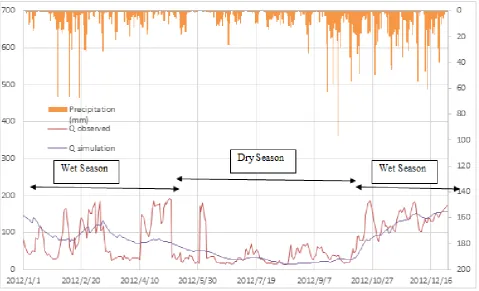
[image:8.595.59.539.366.657.2]The hydrograph results of scenario 1 were presented in Figure 7. This hydrograph shows that the fluctuation of water level was a function of rain fall (orange line). During the rainy season in the period of January to April, and October to December, it showed that there was a trend that the river water level (red line) was relatively higher compared to those in the dry season period (May to September 2012). However, in this case, the global climate change and El-Nino effect were not put into an account in this scenario.
Figure 7. Hydrograph model for the year 2012 developed using the SWAT
Scenario 2. After Conservation
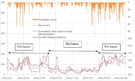
[image:9.595.63.537.147.432.2]Based on the SWAT simulation, after conducting the conservation program, it was revealed that the determination coefficient (R2) was 0.50 > 0.4 and NS was 0.5 > 0.36 (green line). Thus this hydrological model for this watershed was also considered acceptable (Figure 8).
Figure 8. Comparison of 3 hydrographs based on Q observation, and 2 models after calibration
It was identified that, the simulated hydrograph (before and after conservation, black and blue lines respectively) were relatively smooth compared to the real conditions; as these simulations take into account statistic approaches which accommodate a certain level of errors [13]. The water balance parameters were calculated using the curve number method [19] for the surface runoff. The Hargreaves method was used for the potential evapotranspiration process [19, 20].
Summary:
No Parameters Existing (2012)
(Scenario 1) Simulation (Scenario 2) Recommendation
1 Percentage of critical land area areas (PLK) 10.41% (moderate or so-so) 6.47% (low or good)
No urgent attention required in managing the watershed as a small number of critical land exist in the scenario 1-2.
2 Percentage of vegetation coverage areas (PPV) 71.6% (good) 73% (good) No urgent attention required in managing the watershed as there is >60% of watershed area was covered by vegetation.
3 Water flow regime coefficient (KRA) 14.58 (very low or very good) 31 (low of good) No urgent attention required in managing the watershed as the fluctuation of river water flow between dray season period and rain one was relatively low.
4 Annual Water flow Coefficient (KAT). 0.45 (high) 0.44 (high) watershed area as the indirect water run-off >40 (high). There is a need special attention in managing the
Based on the summary table above, there was identified that after conducting replanting (reforestation) programs, there were identified an improvement of the watershed performances, however there is a urgent attention for expanding reforestation areas in order to reduce the annual water flow coefficient to become < 0.30 (based on the standard of the Minister of Forestry of the Republic of Indonesia Decree, 2014, and Directorate General of Land and Social Forestry Annex no. P.04/V-Set/2009) [9, 10].
4. Conclusions
The combination of remote sensing (RS) data obtained from the Landsat ETM+ and GIS application have yield land cover maps of the sub-Siak watershed for 2002, 2007 and 2012. Based on the watershed existing condition (scenario 1), it was identified that Percentage of critical land area areas (PLK) value was 10.41%, the percentage of vegetation coverage areas (PPV) 71.6%, the water flow regime coefficient (KRA) 14.58, and the annual water flow coefficient (KAT) 0.45. After an application of the conservation scheme (scenario 2) the condition of the watershed including PLK improve by 37%, PPV 2%, KRA 60%, and KAT 2%. These values show that the overall watershed performances in the scenario 2 were better than those in the scenario 1. This study recommended to conduct reforestation programs in order to reduce the annual water flow coefficient to become less than 0.30 (low) The hydrograph simulation model for this watershed was also considered acceptable as the determination coefficient (R2) was 0.50 > 0.4 and NS was 0.5 > 0.36.
Acknowledgements
We would like to thank the Civil Engineering Faculty, Universitas Riau and Research and Development Board (Balitbangda), Riau Province, Indonesia for technically
facilitating this research study.
REFERENCES
[1] Yesi Gusriani, 2012, A Strategy for Managing of Water Pollution in Siak Watershed (Strategi Pengendalian Pencemaran Daerah Aliran Sungai (Das) Siak), Kabupaten Siak, Program Studi Ilmu Administrasi Negara FISIP Universitas Riau, Pekanbaru, 2-3.
[2] Fatimah Ratna Sari and Denny Zulkaidi, 2014. Managing Zonation Principles for Developing River Area (Prinsip Pengaturan Zonasi Untuk Pengembangan Kawasan Tepi Sungai), Studi Kasus: Sungai Siak, Kota Pekanbaru, Jurnal Perencanaan Wilayah dan Kota,Vol. 2, No. 2, Sekolah Arsitektur, Perencanaan dan Pengembangan Kebijakan ITB, 211-219.
[3] Asdak, C., 1995, Hydrology and Watershed Management (Hidrologi dan Pengelolaan Daerah Aliran Sungai). Yogyakarta: Gadjah Mada University Press, 25-40.
[4] Cohen Liechti, T. et al. 2014. “Hydraulic–hydrologic Model for Water Resources Management of the Zambezi Basin.” Journal of Applied Water Engineering and Research 2(2): 105–17.
http://www.tandfonline.com/doi/abs/10.1080/23249676.201 4.958581.
[5] Ridwansyah, Iwan, Hidayat Pawitan, Naik Sinukaban, and Yayat Hidayat. 2014. “Watershed Modeling with ArcSWAT and SUFI2 In Cisadane Catchment Area: Calibration and Validation of River Flow Prediction.” International Journal of Science and Engineering 6(2): xx.
[6] Arnold, J.G., R. Srinivasan, R.S. Muttiah, and J.R. Williams. 1998. Large area hydrologic modeling and assessment Part I: Model Development. Journal of the American Water Resources Association, 34(1): 73-89.
[8] Ari Sandhyavitri, et all, 2015. The Changes of Land Use Pattern Affect to the Availability of Water Resources in Siak Watershed, Riau Province, Indonesia, Proceeding of the 14th International Conference on QIR (Quality in Research), Lombok, Indonesia, 10-13 August 2015, ISSN 1411-1284, 208-213.
[9] The Minister of Forestry of the Republic of Indonesia Decree, 2014, Number: P. 61 / Menhut II / 2014 concerning A Guideline for Monitoring and Evaluation of Watershed. 7-15.
[10]Directorate General of Land and Social Forestry Annex no. P.04/V-Set/2009. A Guideline for Monitoring and Evaluation of Watershed. 75-78.
[11]BPDAS, 2012, Siak Watershed Land Cover, Riau, Indonesia, 2-12.
[12]ASTER GDEM (Global Digital Elevation Model) with a resolution of 30 m. It may be downloaded from
http://gdem.ersdac.jspacesystems.or.jp/ and http://www.jspacesystems.or.jp/ersdac/GDEM/E/4.html
[13]Neitsch SL, et all. 2005. Soil and Water Assessment Tool, Theorical Documentation Version 2005. Grassland Soil and Water Research Laboratory, Agricultural Research Service, Blackland Research Center- Texas Agricultural Experiment Station. USA.
[14]Arnold, J. G. et al. 2012. “Swat: Model Use, Calibration, and Validation.” Asabe 55(4): 1491–1508.
[15]Migliaccio, K.W., and P. Srivastava, 2007. Hydrologic components of watershed-scale models. Transactions of the ASAE, 50(5): 1695-1703.
[16]Hambali, R. 2008. Water Potential Analyses using Mock Model (Analisis Ketersediaan Air dengan Model Mock). Bahan Ajar. Yogyakarta: Universitas Gadjah Mada
[17]Motovilov, Y.G., Gottschalk, L., Engeland, K. & Rodhe, A. 1999. Validation of a Distributed Hydrological Model against Spatial Observations. Elsevier Agricultural and Forest Meteorology. 98: 257-277.
[18]R. Rosso, A. Peano, I. Becchi and G. A. Bemporad, 1994, An Introduction to Spatially Distributed Modelling of Basin Response,” Water Resources Publications, Highland Ranch. 3-30.
[19]D. C. Garen and D. S. Moore, 2005, Curve Number Hydrology in Water Quality Modeling: Uses, Abuses, and Future Directions, Journal of the American Water Resources Association, Vol. 41, No. 2, pp. 377-388

![Table 1. Evaluation Criteria for Watershed Performances [9,10].](https://thumb-us.123doks.com/thumbv2/123dok_us/8790328.908972/4.595.86.509.468.733/table-evaluation-criteria-watershed-performances.webp)