Analysis of Variance of Cross-Validation Estimators of the
Generalization Error
Marianthi Markatou [email protected]
Hong Tian [email protected]
Department of Biostatistics Columbia University New York, NY 10032, USA
Shameek Biswas [email protected]
George Hripcsak [email protected]
Department of Biomedical Informatics Columbia University
New York, NY 10032, USA
Editor: David Madigan
Abstract
This paper brings together methods from two different disciplines: statistics and machine learn-ing. We address the problem of estimating the variance of cross-validation (CV) estimators of the generalization error. In particular, we approach the problem of variance estimation of the CV estimators of generalization error as a problem in approximating the moments of a statistic. The approximation illustrates the role of training and test sets in the performance of the algorithm. It provides a unifying approach to evaluation of various methods used in obtaining training and test sets and it takes into account the variability due to different training and test sets. For the simple problem of predicting the sample mean and in the case of smooth loss functions, we show that the variance of the CV estimator of the generalization error is a function of the moments of the random variables Y =Card(SjTSj0)and Y∗=Card(ScjTScj0), where Sj, Sj0 are two training sets, and Scj,
Scj0 are the corresponding test sets. We prove that the distribution of Y and Y* is hypergeometric
and we compare our estimator with the one proposed by Nadeau and Bengio (2003). We extend these results in the regression case and the case of absolute error loss, and indicate how the methods can be extended to the classification case. We illustrate the results through simulation.
Keywords: cross-validation, generalization error, moment approximation, prediction, variance estimation
1. Introduction
Progress in digital data acquisition and storage technology has resulted in the growth of very large databases. At the same time, interest has grown in the possibility of tapping these data and of extracting information from the data that might be of value to the owner of the database. A variety of algorithms have been developed to mine through these databases with the purpose of uncovering interesting characteristics of the data and generalizing the findings to other data sets.
indepen-dent test data. The assessment of the performance of learning algorithms is extremely important in practice because it guides the choice of learning methods.
The generalization error of a learning method can be easily estimated via either cross-validation or bootstrap. However, providing a variance estimate of the estimator of this generalization error is a more difficult problem. This is because the generalization error depends on the loss function involved, and the mathematics needed to analyze the variance of the estimator are complicated. An estimator of variance of the cross-validation estimator of the generalization error is proposed by Nadeau and Bengio (2003). In a later section of this paper we will discuss this estimator and compare it with the newly proposed estimator.
In this paper we address estimation of the variance of the cross validation estimator of the generalization error, using the method of moment approximation. The idea is simple. The cross validation estimator of the generalization error is viewed as a statistic. As such, it has a distribution. We then approximate the needed moments of this distribution in order to obtain an estimate of the variance. We present a framework that allows computation of the variance estimator of the generalization error for k fold cross validation, as well as the usual random set selection in cross validation. We address the problem of loss function selection and we show that for a general class of loss functions, the class of differentiable loss functions with certain tail behavior, and for the simple problem of prediction of the sample mean, the variance of the cross validation estimator of the generalization error depends on the expectation of the random variables Y =Card(SjTSj0)
and Y∗=Card(ScjT
Scj0). Here Sj, Sj0 are two different training sets drawn randomly from the data
universe and Scj, Scj0 are their corresponding test sets taken to be the complement of Sj and Sj0 with
respect to the data universe. We then obtain variance estimators of the generalization error for the k-fold cross validation estimator, and extend the results to the regression case. We also indicate how the results can be extended to the classification case.
The paper is organized as follows. Section 2 introduces the framework and discusses existing literature on the problem of variance estimation of the cross validation estimators of the generaliza-tion error. Secgeneraliza-tion 3 presents the moment approximageneraliza-tion method for developing the new estimator. Section 4 presents computer experiments and compares our estimator with the estimator proposed by Nadeau and Bengio (2003). Section 5 presents discussion and conclusions.
2. Framework and Related Work
In what follows we describe the framework within which we will work.
2.1 The Framework and the Cross Validation Estimator of the Generalization Error
Let data X1,X2,···,Xn be collected such that the data universe, Z1n={X1,X2,···,Xn}, is a set of
independent, identically distributed observations which follow an unknown probability distribution, denoted by F. Let S represent a subset of size n1, n1<n, taken from Zn1. This subset of observations
is called a training set; on the basis of a training set a rule is constructed. The test set contains all data that do not belong in S, that is the test set is the set Sc=Z1n\S, the complement of S with respect to the data universe Z1n. Denote by n2the number of elements in a test set, n2=n−n1, n2<n.
Let L :Rp×R→Rbe a function, and assume that Y is a target variable and ˆf(x)is a decision
As an example, consider the estimation of the sample mean. In this problem the learning algo-rithm uses ˆf(x) =n1
1∑
n1
i=1Xi=X¯Sj as a decision rule and L(X¯Sj,Xi) = (X¯Sj−Xi) 2, X
i∈Scj, the square
error loss, as a loss function. Other typical choices of the loss function include the absolute error loss,|X¯S
j−Xi|and the 0−1 loss function mainly used in classification.
Our results take into account the variability in both training and test sets. The variance estimate of the cross validation estimator of the generalization error can be computed under the following cross validation schemes. The first is what we term as complete random selection. When this form of cross validation is used to compute the estimate of the generalization error of a learning method, the training sets, and hence the test sets, are randomly selected from the available data universe. In the nonoverlapping test set selection case, the data universe is divided into k nonoverlapping data subsets. Each data subset is then used as a test set, with the remaining data acting as a training set. This is the case of k-fold cross validation.
We now describe in detail the cross validation estimator of the generalization error whose vari-ance we will study. This estimator is constructed under the complete random selection case.
Let Aj be a random set of n1 distinct integers from {1,2,···,n}, n1 <n. Let n2 =n−n1
be the size of the corresponding complement set. Note here that n2 is a fixed number and that
Card(Aj) =n1 is fixed. Let A1,A2,···,AJ be random index sets sampled independently of each
other and denote by Acj, the complement of Aj, j=1,2,···,J. Denote also by Sj={Xl : l∈Aj},
j=1,2,···,J. This is the training set obtained by subsampling Z1naccording to the random index set Aj. Then the corresponding test set is Scj={Xl : l∈Acj}. Now define L(j,i) =L(Sj,Xi), where
L is a loss function. Notice that L is defined by its dependence on the training set Sjand the test set
Scj. This dependence on the training and test sets is through the statistics that are computed using the elements of these sets. The usual average test set error is then
ˆµj=
1 n2i
∑
∈Scj
L(j,i), (2.1)
The cross validation estimator we will study is defined as
n2
n1ˆµJ = 1 J
J
∑
j=1ˆµj. (2.2)
This version of the cross validation estimator of the generalization error depends on the value of J, the size of the training and test sets and the size of the data universe. The estimator has been studied by Nadeau and Bengio (2003). These authors provided two estimators of the variance of
n2
n1ˆµJ. In the next section we review briefly the estimators presented by Nadeau and Bengio (2003) as well as other work on this subject. In a later section we will see that, when J is chosen appropriately, then the Nadeau and Bengio (2003) estimator is close to and performs similarly with the moment approximation estimator in some of the cases we study.
2.2 Related Work
Related literature for the problem of estimating the variance of the generalization error includes work by McLachlan (1972, 1973, 1974, 1976) and work by Nadeau and Bengio (2003) and Bengio and Grandvalet (2004). Here, we briefly review this work.
Let S2ˆµj = J−11∑Jj=1(ˆµj−nn21ˆµJ)
2be the sample variance of ˆµ
j, j=1,2,···,J. Then Nadeau and
E(S2ˆµj) =Var( n2
n1ˆµJ)
(1J+1−ρρ), (2.3)
whereρis the correlation between ˆµjand ˆµj0. Therefore, ifρis known,
(1
J+
ρ
1−ρ)S
2
ˆµj, (2.4)
is an unbiased estimator of the Var(n2
n1ˆµJ). Nadeau and Bengio (2003) observe that this estimator depends on the correlationρ between the different ˆµjs which is difficult to estimate. Thus, they
propose an approximation to the correlation, ˆρ=n2
n, where n2is the cardinality of the test set. The
final estimator of the variance ofn2
n1ˆµJ is given as
(1
J+ n2
n1
)S2ˆµj. (2.5)
Nadeau and Bengio (2003) note that the above suggested estimator is simple but it may have a positive or negative bias with respect to the actual Var(n2
n1ˆµJ). That is, it will tend to overestimate or underestimate Var(n2
n1ˆµJ)according to whether ˆρ=
n2
n >ρor ˆρ<ρ. Therefore, this estimator is not
exactly unbiased.
Nadeau and Bengio (2003) also suggested another estimator of the variance of the cross-validation estimator of the generalization error. This estimator is unbiased but overestimates the Var(n2
n1ˆµJ). It is computed as follows. Let n be the size of the data universe and assume, without loss of general-ity, that n is even. Randomly split the data set into two, equal size, data subsets. Then compute the cross-validation estimator of the generalization error on these two data subsets. Notice that, the size of the training set is now n01= [n2]−n2<n1, smaller than the original size of the training set, but the
test set size remains the same. Denote by ˆµ1the estimatornn20
1ˆµJ computed on the first data subset and ˆµ2the estimatornn20
1ˆµJ computed on the second data subset. To obtain an estimator of the variance of the cross validation estimator of the generalization error compute the sample variance of ˆµ1and ˆµ2.
The splitting process can be repeated M times and Nadeau and Bengio(2003) recommend M=10. The proposed unbiased estimator is then given as
1 2M
M
∑
m=1(ˆµ1,m−ˆµ2,m)2. (2.6)
This is an unbiased estimator of the Var(n2
n0
1ˆµJ).
Bengio and Grandvalet (2004) showed that there does not exist any unbiased and universal estimator of the variance of k-fold cross-validation that is valid under all distributions. Here, we derive estimators of the variance of the k-fold cross validation estimator of the generalization error that are almost unbiased. However, we also notice that our estimators do depend on the distribution of the errors and on the knowledge of the learning algorithm.
rate and risk associated with Anderson’s classification statistic in the context of the two-population discrimination problem. These derivations were carried out under the assumption of normality for the population distribution.
Our work has similarities with the work by McLachlan in the sense that we derive approxima-tions to the moments of the distribution of the cross validation estimator of the generalization error and use these to obtain a variance estimator. However, we do not assume normality of the underly-ing mechanism that generated the data.
In what follows, we first present the method of moment approximation for obtaining an estima-tor of Var(n2
n1ˆµJ). We then study the performance of this estimator and compare it with the Nadeau and Bengio (2003) estimator.
3. Moment Approximation Estimator for Var(n2 n1ˆµJ)
Recall thatn2
n1ˆµJ =
1 J∑
J
j=1ˆµj =1J∑Jj=1(n12∑i∈S
c
jL(j,i)). Therefore n2
n1ˆµJ is a statistic. An estimator of Var(n2
n1ˆµJ) can thus be obtained by approximating the moments of the statistic
n2
n1ˆµJ. A simple calculation shows that
Var(n2
n1ˆµJ) = 1 J2
J
∑
j=1Var(ˆµj) +
1 J2
∑ ∑
j6=j0
Cov(ˆµj,ˆµj0). (3.1)
From the formula we see that if we can approximate the two terms of(3.1) then we can obtain an estimator for the variance ofn2
n1ˆµJ. To achieve this goal, we need to estimate E(ˆµj), E(ˆµ
2 j)and
E(ˆµjˆµj0). In the following sections we will develop the theory that allows us to obtain the needed
moment approximations. To illustrate the methodology clearly we treat separately the case of simple mean estimation and the regression case. We further treat separately the case where the loss function is differentiable from the case of non-differentiable loss functions.
3.1 The Sample Mean Case
We start by analyzing the case of the sample mean. Here, the loss function L depends on Sjthrough
the statistics ¯XSj, the sample mean computed using the elements of Sj, and on S c
j by elements
Xi∈Scj. One of the reasons for presenting the sample mean case separately is because it illustrates
clearly the contribution towards the estimator of Var(n2
n1ˆµJ)that is due to the variability among the different training and test sets. A second reason in favor of this case is because, under square error loss, we obtain a “ golden standard” against which we can compare the new empirically computed variance estimator and the Nadeau and Bengio (2003) estimator. This “golden standard” is the exact theoretical value of the Var(n2
n1ˆµJ). The obtained results show that the estimator of the variance of the cross validation estimator of the generalization error of the algorithms that use differentiable functions of the mean as loss functions, depends on the expectation of the random variables Y =
Card(SjTSj0)and Y∗=Card(ScjTScj0).
Let the loss function L(j,i) =L(X¯S
j; Xi)be differentiable. Below we list the conditions under which our theory holds.
Assumption 1. The distribution of L(X¯S
Assumption 2. The loss function L as a function of ¯XSj is such that its first four derivatives with respect to the first argument exist for all values of the variable that belongs in I, where I is an interval such that P(v∈I) =1, and v indicates the first argument of the loss function.
Assumption 3. The fourth derivative of L is such that|L(iv)(X¯S
j; Xi)| ≤M(Xi), E[M(Xi)]<∞. Assumption 1 is also used by Nadeau and Bengio (2003, p. 244). Assumptions 2 and 3 are standard in the literature where approximations to the moments of a continuous, real function of the mean are discussed. See, for example Cramer (1946), Lehmman (1991) and Bickel and Doksum (2001). The boundedness of the fourth or some higher derivative is necessary for proposition 3.1 to hold.
Alternative conditions where stronger assumptions on the distributions of the data Xiand weaker
conditions on the function L are imposed exist in the literature (Khan (2004)). Here L is a loss func-tion and it seems reasonable to assume boundedness on some of its higher derivatives.
Proposition 3.1 offers an approximation of the expectation of L(X¯S j,Xi).
Proposition 3.1 Let X1,X2,···,Xnbe independent, identically distributed random variables such
that E(Xi) =µ, Var(Xi) =σ2 and finite fourth moment. Suppose that L satisfies assumptions 1, 2
and 3. Then
E[L(X¯Sj; Xi)] =E[L(µ,Xi)] +
σ2
2n1
E[(L00(µ,Xi))] +O(
1 n21), where the remainder Rn is such that E(Rn) is O(n12
1
), that is, there exists n0 and A<∞such that
E(Rn)< nA2 1
,∀n>n0and all µ. The prime indicates derivative with respect to the first argument of
L.
Proof: We will use a conditional expectation argument. Write
E[L(X¯S
j; Xi)] =ESj,i{EZn1[L(X¯Sj; Xi)|Sj,i]}, (3.2)
j=1,2,···,J and i indicates Xiand is such that i∈Scj.
Now expand L(X¯S
j; Xi)with respect to ¯XSj around the mean µ to obtain:
L(X¯Sj; Xi) = L(µ,Xi) +L0(µ,Xi)(X¯Sj−µ) + 1 2L
00(µ,X
i)(X¯Sj−µ) 2 + 1
6L
000(µ,X
i)(X¯Sj−µ) 3+ 1
24L
(iv)(µ∗,X
i)(X¯Sj−µ)
4. (3.3)
Denote by
Rn=L(iv)(µ∗,Xi)(X¯Sj−µ) 4
and
EZn
1{Rn|Sj,i}=EZ1n{L
(iv)(µ∗,X
i)(X¯Sj−µ) 4|S
j,i}, (3.4)
and since by assumption 1 the distribution of L(iv)(µ∗,Xi)(X¯Sj−µ)
4does not depend on the particular
realization of Sjand i, we obtain
ESj,i{EZ1n[L
(iv)(µ∗,X
i)(X¯Sj−µ) 4
|Sj,i]}=E[L(iv)(µ∗,Xi)]E(X¯Sj−µ) 4
≤M·E(X¯S j−µ)
This is because by assumption 3 we have E[L(iv)(µ∗,Xi)]≤E[M(Xi)]<∞. Now Lemma A.5 of the
appendix guarantees that E(X¯S j−µ)
4is of order 1/n2
1. Thus, taking expectations in (3.3) and using
(3.4) we obtain:
E[L(X¯S
j; Xi)] = ESj,i{EZ1n[L(µ,Xi)|Sj,i]}+ESj,i{EZ1n[L
0(µ,X
i)(X¯Sj−µ)|Sj,i]}
+ ESj,i{EZ1n[ 1 2L
00(µ,X
i)(X¯Sj−µ) 2|S
j,i]} + ESj,i{EZ1n[
1 6L
000(µ,X
i)(X¯Sj−µ) 3
|Sj,i]}+O(
1 n21).
By assumption 1 the distribution of L(µ,Xi)does not depend on the particular realization of Sjand
Xi. Thus
ESj,i{EZ1n[L(µ,Xi)|Sj,i]}=EZ1n[L(µ,Xi)].
Similar to the above arguments produce the approximation to the first moment given by
E[L(X¯S
j; Xi)] =E[L(µ,Xi)] +
σ2
2n1
E[(L00(µ,Xi))] +O(
1 n21).
Remark 1: Note that we do not impose distributional assumptions on the data. The only
condi-tion imposed is that samples come from distribucondi-tions for which the fourth moment is finite. Many of the standard families of distributions satisfy this condition.
Remark 2: The requirement of the finiteness of the fourth moment for proposition 3.1 to hold
implies limitations on the data sets on which this estimator can be computed. For example, it may be inappropriate to apply these methods to data sets which involve large variations, such as those from insurance and finance. On the other hand, the results apply to some thick tail distributions, such as the t-distribution with 5 or more degrees of freedom. The t5-distribution, for example, is a
thick tail distribution, for which the fourth moment exists.
The following proposition approximates the variance of the loss L(X¯S j,Xi).
Proposition 3.2 Let assumptions 1, 2 and 3 hold. If in addition the fourth derivative of L2(X¯S j,Xi) is bounded, then
Var[L(X¯S
j; Xi)] =Var[L(µ,Xi)] +
σ2
n1{
E[(L0(µ,Xi))2] +Cov(L(µ,Xi),L00(µ,Xi))}+O(1/n21),
where the remainder term is O(1 n2 1
).
Proof: To obtain an expansion of the variance of L(X¯S
j; Xi)apply proposition 1 to the function
L2(X¯S
j; Xi)using the fact that
[L2(µ,Xi)]00 =
∂2
∂µ2[L 2(µ; X
i)]
Then substituting the expansion for L(X¯S
j,Xi)and using formula (3.5), proposition 1 and the formula of conditional variance we obtain:
Var[L(X¯S
j; Xi)] =Var[L(µ,Xi)] +
σ2
n1{
E[(L0(µ,Xi))2] +Cov(L(µ,Xi),L00(µ,Xi))}+O(1/n21).
To prove the above two propositions we use a series of lemmas that guarantee the rate of the remainder term. These lemmas are presented in the appendix.
We now present a theoretical example that verifies the approximations presented in propositions 1 and 2.
Example. Assume that L(X¯S
j,Xi) = (X¯Sj−Xi)
2, the square error loss that is widely used. An
exact calculation of the expectation of(X¯S j−Xi)
2produces
E{L(X¯S
j,Xi)}=Var(X¯Sj) +Var(Xi) =σ 2+σ2
n1 .
On the other hand, if proposition 3.1 is used, we obtain:
E[L(X¯S
j,Xi)] =E(Xi−µ) 2+σ2
n1
=σ2+σ2
n1 ,
and the two formulas coincide. Notice that in the case of square error loss, the second derivative of the loss, with respect to µ, is bounded. The terms of order 1/n21do not enter the formula as all higher order than two derivatives of the quadratic loss are 0. Thus, the approximation formula agrees with the exact computation.
We next turn to the variance formula. The exact computation is based on the formula
Var[L(X¯S
j,Xi)] =ESj,i{VarZ1n[(X¯Sj−Xi) 2
|Sj,i]}+VarSj,i{EZn1[(X¯Sj−Xi) 2
|Sj,i]}. (3.6)
Using this formula we obtain the exact variance as
Var[L(X¯S
j,Xi)] =2σ 4+4σ4
n1 +2σ
4
n2 1
. (3.7)
Using the formula given in proposition 3.2 we obtain that the approximate variance is
Var[L(j,i)] =2σ4+4σ 4
n1
+O(1
n21). (3.8)
Comparing these two formulas we see that the variance approximation formula identifies all first order terms.
The following proposition establishes the approximation formula for the covariance terms that enter the computation of the variance of the cross validation estimators of the generalization error.
Proposition 3.3 Let Sj, Sj0 be two training sets drawn independently and at random from the
data universe Z1n, and Scj, Scj0 the corresponding test sets. Let Xi ∈Scj,Xi0 ∈Scj0, D=SjTSj0 and
Y =Card(D). Then, if i6=i0
Cov[L(X¯S
j,Xi),L(X¯Sj0,Xi0)] =
σ2
n2 1
E(Y)(E[L0(µ,Xi)])2−
σ4
4n2 1
(E[L00(µ,Xi)])2+O(
1 n2
If i=i0,
Cov[L(X¯S
j,Xi),L(X¯Sj0,Xi0)] = Var(L(µ,Xi)) +
σ2
n1{
E[L(µ,Xi)L00(ξ,i)]
− E[L(µ,Xi)]E[L00(µ,Xi)]}+
σ2
n21E(Y)E[L
0(µ,X
i)]2
− σ
4
4n21{E[L
00(µ,X
i)]}2+O(
1 n21),
where E(Y)is the expectation of the random variable Y with respect to its distribution.
This proposition indicates that the variability due to random sampling of the training sets Sj is
quantified by the expectation of the random variable Y =Card(SjTSj0), j6= j0, j,j0∈1,2,···,J.
Since Sj, Sj0 are random sets of n1elements, Y is such that max(0,2n1−n)≤Y ≤n1.
An additional random variable that enters the variance estimator of the cross validation esti-mator of the generalization error is Y∗=Card(ScjT
Scj0), the cardinality of the intersection of two
different test sets. The following two lemmas derive the distribution of these two random variables.
Lemma 3.1 Let Sjand Sj0be random sets of n1distinct elements from Z!nand let Y=Card(SjTScj),
max(0,2n1−n)≤Y ≤n1. Then, the distribution of Y is
P(Y=y) = n1
y
n−n1
n1−y
n n1
,
a hypergeometric distribution.
Proof. We model the problem as the following 2×n table.
k 1 2 3 ··· n Total
Sj 0 1 1 ··· 0 n1
Sj0 1 0 1 ··· 0 n1
a1 a2 a3 ··· an 2n1
In the table we indicate whether the kth component of Z1nis sampled into the training set Sj or Sj0
by 1, otherwise we indicate it by 0. Denote by akthe sum of the indicators for the kth component in
the population Z1nover Sjand Sj0. Then
a1+a2+···+an=2n1
0≤ai≤2 ,i=1,···,n.
Now, P(Y =y)is equivalent to P(#{ai =2}), i=1,···,n. Given Y =y, the number of{ai =1}
is 2n1−2y and the number of{ai =0} is n−2n1+y. Since none of these three numbers could
be negative, we obtain the domain of Y as max(0,2n1−n)≤Y ≤n1. Recall also that Sj, Sj0 are
sampled independently and each contains n1elements. Given Y=y, the distribution of the column
totals is fixed; that is ai can only take the values 0 ,1 or 2. The number of different tables with the
same column totals is then ny n−y n1−y
n−n1
n1−y
. and hence
P(Y =y) = n y
n−y n1−y
n−n1
n1−y
n n1
n
n1
=
n1
y
n−n1
n1−y
n n1
the hypergeometric distribution.
Lemma 3.2 Let Sj and Sj0 be two training sets and Scj and Scj0 are their corresponding test sets.
Let Y∗=Card(ScjT
Scj0), 0≤Y∗≤n−n1. Then
P(Y∗=y) = n1
y−n+2n1
n−n1
n−n1−y
n n1
=
n2
n2−y
n−n2
n−n2−(n2−y)
n n−n2
.
Proof. From the proof of lemma 3.1 P(Y∗ =y) =P(#{ai =0}), {i=1,···,n}. Moreover,
Y∗=n−2n1+Y . Then, the result follows.
Theorem 3.1 provides the estimator of the variance ofn2
n1ˆµJ. We first state the theorem.
Theorem 3.1. The variance of the estimator of the generalization errorn2
n1ˆµJis given as Var(n2
n1ˆµJ) = 1
JVar(ˆµj) + J−1
J Cov(ˆµj,ˆµj0), where
Var(ˆµj) =
1 n2
[Var[L(µ,Xi)] +
σ2
n1{
E[(L0(µ,Xi))2] +Cov(L(µ,Xi),L00(µ,Xi))}] + n2−1
n2
σ2
n1{
E[L0(µ,Xi)]}2+O(1/n21),
Cov(ˆµj,ˆµj0) = (1−E(Y
∗)
n22 )
hσ2
n21E(Y)(E[L
0(µ,X
i)])2−
σ4
4n21(E[L
00(µ,X
i)])2+O(
1 n21)
i
+ E(Y∗)
n2 2
h
Var(L(µ,Xi)) +
σ2
n1{
E[L(µ,Xi)L00(µ,Xi)]−E[L(µ,Xi)]E[L00(µ,Xi)]}
+ σ 2
n21E(Y)E[L
0(µ,X
i)]2−
σ4
4n21{E[L
00(µ,X
i)]}2+O(
1 n21)
i
,
where µ=EZn
1Xi,σ
2=Var Zn
1(Xi).
The above formulas indicate clearly the dependence of Var(n2
n1ˆµJ) on the first moment of the random variables Y , Y∗. Since the distribution of Y and Y∗is known, we can substitute E(Y), E(Y∗)
by their corresponding values and simplify the above expressions. Because the distribution of Y , Y∗ is hypergeometric E(Y) =n21
n and E(Y∗) = n2
2
n. Then
Cov(ˆµj,ˆµj0) = (1−1
n)
hσ2
n (E[L
0(µ,X
i)])2−
σ4
4n21(E[L
00(µ,X
i)])2+O(
1 n21)
i
+ 1
n
h
Var(L(µ,Xi)) +
σ2
n1{
Cov(L(µ,Xi),L00(µ,Xi))}
+ σ 2
n E[L
0(µ,X
i)]2−
σ4
4n2 1
(E[L00(µ,Xi)])2+O(
1 n2
The final estimator of the variance of n2
n1ˆµJ is a plug-in estimator and it can be computed using theorem (3.1). We need to replace the unknown population mean µ and population variance σ2 by their estimators, the sample mean and sample variance respectively. If it is not convenient to compute the sample variance and mean based on the data universe we may compute ¯XSj and, if there are many different training sets, take as an estimator of the sample mean ¯X = 1
J∑ J j=1X¯Sj. Moreover, ˆσ2j = 1
n1−1∑
n1
l=1(Xl−X¯Sj)
2, thus the variance estimate of the population variance will be
ˆ
σ2=1 J∑
J j=1σˆ2j.
Example. In the case of square error loss the approximations to the variance of ˆµj and the
Cov(ˆµj,ˆµj0)are given as:
Var(ˆµj) =
1 n2
Var[(Xi−µ)2] +
4σ4 n1n2
= 1
n2
E[(xi−µ)4]−σ 4
n2 + 4σ
4
n1n2
, (3.9)
Cov(ˆµj,ˆµj0) = (1−1
n)(−
σ4
n21) + 1 n(
4σ4
n −
σ4
n21 +Var[(Xi−µ)
2]). (3.10)
If the data are from a N(0,σ2)then the moment approximation estimator of the variance ofn2
n1ˆµJ is given by
ˆ
σ4{2(n1+2)
n1n2
1 J + (
J−1 J )[
2(n+2)
n2 −
1 n2
1 ]},
where ˆσis the sample standard deviation. Thus the estimator of the variancen2
n1ˆµJ is a multiple of the sample variance and the multiplication factor indicates the dependence of the estimator on n1, n2and n.
Variance estimator of the k-fold CV estimator of the generalization error.
Here we present a variance estimator of the k-fold cross validation estimator of the general-ization error of a learning algorithm. Notice that this is a special case of theorem 3.1. In k-fold cross validation the data universe is divided into k different non-overlapping test sets, each of which contains nk elements. The number of elements n1, in any given training set, is then n−nk =(k−k1)n.
Therefore, Y =Card(SjTSj0) =(k−k2)n. Theorem 3.1 gives the approximations:
Var(ˆµj) =
k
n[Var(L(µ,Xi)) +
σ2
n ( k
k−1){E[(L
0(µ,X
i))2] +Cov(L(µ,Xi),L00(µ,Xi))}] + n−k
n
σ2
n k k−1{E[L
0(µ,X
i)]}2+O(1/n21),
and
Cov(ˆµj,ˆµj0) = σ
2
n
k(k−2)
(k−1)2(E[L0(µ,Xi)]) 2− σ4
4n2(
k k−1)
2(E[L00(µ,X
i)])2+O(
1 n2
1 ).
Therefore, the variance estimate can be computed using relation (3.1), where Var(ˆµj)and Cov(ˆµj,ˆµj0)
are replaced by their estimates. These can be obtained by replacing µ,σ2by their sample estimates
Now assume that the loss function used is square error. In this case, L0(µ,xi) =2(µ−xi)and
L00(µ,xi) =2. The formulas then for the variance of ˆµj and the covariance between different ˆµjs
simplify as follows:
Var(ˆµj) =
k
n{Var[(Xi−µ)
2] +4σ4
n ( k
k−1)}, (3.11)
Cov(ˆµj,ˆµj0) =−σ
4
n2(
k k−1)
2, j
6
= j0. (3.12)
Then Var(n2
n1ˆµJ)can be estimated by using formula (3.1) and replacingσ
2and Var[(X
i−µ)2]by the
sample variance and an appropriate sample estimate for Var[(Xi−µ)2]. The final approximation of
the variance ofn2
n1ˆµJ is then
Var(n2
n1ˆµJ) = 1
n{Var[(Xi−µ)
2]}+ 3kσ4 (k−1)n2 =
1
nE[(Xi−µ)
4]−σ4
n +
3kσ4 (k−1)n2.
A simple estimator of E[(Xi−µ)4]can be computed from the training sample by taking the sample
version of the above expectation, n1
1∑i∈Sj(Xi− ¯ XSj)
4. To illustrate, if we further assume a normal
population then Var[(Xi−µ)2] =2σ4and the variance estimator ofnn21ˆµJ is given as ˆ
σ4
n (2+ 3k n(k−1)),
where ˆσis the sample standard deviation.
3.2 The Regression Case
The regression case is another case of fitting means. We consider here the problem of estimat-ing the variance of the cross validation estimator of the generalization error n2
n1ˆµJ in the case of regression. Therefore the data are realizations of random variables(Yi,Xi), i=1,2,···,n such that
E(Yi|Xi) =xTi β. Notice that the explanatory variables here are treated as fixed; this formulation is
known as the fixed design case. The vector of unknown parametersβis usually estimated by least squares; denote by ˆβthe least square estimator ofβ. Then for a new observation(yi,xi)∈Scjdenote
by ˆyi,Sj =x T
i βˆSj, where ˆβSj indicates the estimator ofβcomputed by using the data in the training set Sj. The loss function L is then dependent on ˆyi,Sj and yi, that is L(yˆi,Sj,yi).
To derive the estimator of Var(n2
n1ˆµJ)we need to use the moment approximation method to ob-tain approximations for the moments of the statisticn2
n1ˆµJ. The idea is the same as in the case of simple mean estimation. That is, the loss function is expanded with respect to its first argument and evaluated at the point E(Yi|Xi) =xTi β0, whereβ0is the true parameter value. In other words, as
before, the expansion is evaluated at the true mean.
We list now the assumptions under which our theory holds.
Assumption 1. If Sj is a training set with n1number of elements
lim
n1→∞ 1 n1
where V is finite and positive definite.
Assumption 2. Let xn1k denote the kth row of the design matrix XSj. Then, for each j= 1,2,···,J,
max
1≤k≤n1 xn1k(X
T SjXSj)−
1x n1k→0 as n1→∞.
Notice that this condition is known as the generalized Noether condition. Under the above conditions√n1(βˆSj−β)converges in distribution to a N(0,σ
2V)random
vari-able.
The following proposition establishes an approximation to the expectation of the loss function L.
Proposition 3.4: Suppose that assumptions 1 and 2 hold. Then
E[L(yˆi,Sj,yi)] =E[L(x T
i β0,yi)] +
σ2
2 E[L
00(xT
i β0,yi)]tr[(xixTi )(XTSjXSj)− 1] +R
n,
where the remainder term is of order O(1 n2 1
), and the prime indicates derivative with respect to the first argument of the loss function.
Proof: First expand L(yˆi,Sj,yi)with respect to the first argument to obtain:
L(yˆi,Sj,yi) = L(x T
i β0,yi) +L0(xTi β0,yi)xTi (βˆSj−β0)
+ 1
2L
00(xT
i β0,yi)(βˆSj−β0) Tx
ixTi (βˆSj−β0) +Rn, (3.13) where Rnindicates the remainder term.
Now
E{L(yˆi,Sj,yi)} = ESj,i{EZ1n[L(yˆi,Sj,yi)|Sj,i]}
= ESj,i{EZ1n[L(x
T
i β0,yi)|Sj,i]}+ESj,i{EZ1n[L
0(xT
i β0,yi)xiT|Sj,i]EZn
1[( ˆ
βSj−β0)|Sj,i]}
+ 1
2ESj,i{EZn1[L
00(xT
i β0,yi)|Sj,i]EZn
1[( ˆ
βSj−β0) Tx
ixTi (βˆSj−β0)|Sj,i]} But the expectation EZn
1[( ˆ
βSj−β0)|Sj,i] =0 because EZ1n( ˆ
βSj|Sj,i) =EZn1( ˆ
βSj) =β0. Also since the distribution of ˆβSj is asymptotically N(β0,σ
2(XT SjXSj)−
1), under assumptions 1 and 2 we obtain:
ESj,i{EZ1n[( ˆ
βSj−β0) Tx
ixTi (βˆSj−β0)|Sj,i]} = EZ1n[( ˆ
βSj−β0) Tx
ixTi (βˆSj−β0)]
= σ2tr[(x
ixTi)(XTSjXSj)− 1],
whereσ2=VarZn
1(Xi), the variance of the sample, and tr(A)stands for the trace of the matrix A. Therefore
E[L(yˆi,Sj,yi)] =E[L(x T
i β0,yi)] +
σ2
2 E[L
00(xT
i β0,yi)]tr[(xixTi )(XTSjXSj)− 1] +R
where the expectations are taken with respect to the distribution of the data. Moreover, Rn is of
ordern12 1 .
Proposition 3.5 establishes the approximation for the variance of L(yˆi,Sj,yi).
Proposition 3.5 Suppose that assumptions 1 and 2 hold. Then Var(L(yˆi,Sj,yi))can be approxi-mated as follows:
Var{L(yˆi,Sj,yi)} = Var[L(x T
i β0,yi)]}+σ2tr[(xixTi )(XTSjXSj)− 1
{Cov(L(xTi β0,yi),
L00(xTi β0,yi)) +E[L0(xiTβ0,yi)]2}+Rn,
whereσ2=Var Zn
1(Yi|Xi)and Rnis the remaining term of order
1 n21 .
Proof: The proof is similar with that of proposition 3.2, in that we apply proposition 3.4 to
L2(yˆi,Sj,yi)and we use the fact that
[L2(yˆi,Sj,yi)]00 = 2L(yˆi,Sj,yi)L00(yˆi,Sj,yi) +2[L0(yˆi,Sj,yi)] 2,
where prime indicates derivative with respect to the first argument of the loss function.
Example. To verify the above approximations we use L(yˆi,Sj,yi) = (yˆi,Sj−yi)
2,the square error
loss and the case of simple regression, that is
yi=a+bzi+εi=xTi β+εi,
where xTi = (1,zi),βT = (a,b)and(yi,xi)∈Scj.The notation ˆyi,Sj stands for x T i βˆSj. The exact expectation of L(yˆi,Sj,yi) = (x
T
i βˆSj−yi)
2is given as:
E[L(yˆi,Sj,yi)] =σ
2+σ2xT
i(XTSjXSj)− 1x
i.
The approximate expectation is
E[L(yˆi,Sj,yi)] =σ
2+σ2tr(x
ixTi (XTSjXSj)
−1),
Because tr(xixTi (XTSjXSj)− 1) =xT
i (XTSjXSj)− 1x
i, the approximation to the expectation agrees with
the exact computation. Similarly we can verify that the approximation of the variance produces the same result as the exact computation. To illustrate further the formulas assume that yi∼N(xTi β,σ2),
then the exact calculation gives the variance of L(yˆi,Sj,yi),
Var(L(yˆi,Sj,yi)) =2σ
4+4σ4xT
i (XTSjXSj)− 1x
i+2σ4(xi(XTSjXSj)− 1x
i)2.
The approximation is given by
Var(L(yˆi,Sj,yi)) =2σ
4+4σ4xT
i (XTSjXSj)− 1x
i+O(
To complete the variance approximation of the estimatorn2
n1ˆµJ we need an approximation of the covariance between L(yˆi,Sj,yi)and L(yˆi0,Sj0,yi0). The following proposition expresses the approxi-mation of Cov(L(yˆi,Sj,yi),L(yˆi,Sj0,yi0)).
Proposition 3.5. Suppose that assumptions 1 and 2 hold. Then for j6= j0, j,j0∈ {1,2,···,J} when i6=i0
Cov(L(yˆi,Sj,yi),L(yˆi0,Sj0,yi0)) =σ
2(E[L0(xT
i β0,yi)])2xTi (XTSj0XSj0)
−1(XT
1X1)(XTSj0XSj0)
−1x
i0
+ σ 4
2 (E[L
00(xT
i β0,yi)])2tr((xixTi )(XTSjXSj)− 1(XT
1X1)(XTSj0XSj0)
−1(x
i0xTi0)
(XTSjXSj)− 1(XT
1X1)(XTSj0XSj0)
−1).
When i=i0,
Cov(L(yˆi,Sj,yi),L(yˆi0,Sj0,yi0)) =Var(L(x T
i β0,yi)) +
σ2
2 Cov(L(x
T
i β0,yi),L00(xTi β0,yi)) (xTi (XTS
j0XSj0)
−1x
i+xTi (XTSjXSj)− 1x
i) + σ2(E[L0(xTi β0,yi)])2xTi (XTSj0XSj0)
−1(XT
1X1)(XTSjXSj)− 1x
i + σ
4
2 (E[L
00(xT
i β0,yi)])2tr((xixTi)(XTSjXSj)− 1(XT
1X1)(XTSj0XSj0)
−1(x
ixTi ) (XTSjXSj)−
1(XT
1X1)(XTSj0XSj0)
−1)
+ σ 4
4Var(L
00(xT
i β0,yi))xTi (XTSjXSj)− 1x
ixTi (XTSj0XSj0)
−1x
i.
Proposition 3.6. Let Sjbe a training set, j=1,2,···,J. Then for i6=i0
Cov(L(yˆi,Sj,yi),L(yˆi0,Sj,yi0)) =σ
2(E[L0(xT
i β0,yi)])2tr[(xi0xiT0)(XTSjXSj)− 1] + σ
4
2 (E[L
00(xT
i β0,yi)])2tr[(xixTi )(XTSjXSj)− 1(x
i0xTi0)(XTSjXSj)− 1].
The proofs of Proposition 3.5 and Proposition 3.6 can be found in Appendix C.
Remark: If the loss is square error,
Cov(L(yˆi,Sj,yi),L(yˆi0,Sj,yi0)) =2σ 4tr[(x
ixTi )(XTSjXSj)− 1(x
i0xTi0)(XTSjXSj)−
1]. (3.14)
To estimate relationship (3.14) we only need to estimateσ. We estimate σby the residual mean square error.
Under square error loss, we have
Var(ˆµj) =
1 n22
n2
∑
i=1{2σ4+4σ4xiT(XTSjXSj)− 1x
i}+
1 n22
∑∑
i6=i02σ4(xTi (XTSjXSj)− 1x
and
Cov(ˆµj,ˆµj0) = 1
n2 2
∑i∈Scj∑i0∈Scj0
i6=i0 {2σ
4tr{(x
ixTi )(XTSjXSj)− 1 (XT1X1)(XTS
j0XSj0)
−1(x
i0xTi0)(XTS
j0XSj0)
−1(XT
1X1)(XTSjXSj)− 1
}}
1 n2
2
∑i∈Sc j∑i0∈Scj0
i=i0 {2σ
4+4σ4xT
i (XTSjXSj)− 1(XT
1X1)(XTSj0XSj0)
−1)x
i +2σ4tr{(xixTi )(XTSjXSj)−
1(XT
1X1)(XTSj0XSj0)
−1(x
ixTi ) (XTS
j0XSj0)
−1(XT
1X1)(XTSjXSj)− 1
}} (3.16)
The final estimate is obtained from relation (3.1) where Var(ˆµj)is estimated by using relation
(3.15), Cov(ˆµj,ˆµj0)is estimated by using relation (3.16) and replacingσ2by an estimator of it. To
obtain an estimator ofσ2, we fit the regression model and obtain ˆyi. Then ˆσ2is the sample variance
of the errors ˆεi=yi−yˆi, that is the residual mean square.
Remark: Note that to derive the results above, we used as the distribution of the data the
conditional distribution of Y given X , in effect treating X as fixed. Now, assume that instead of using the conditional distribution as the data distribution, we treat X as random and use the joint distribution of(X,Y). In this case, the data distribution is
f(x,y) =g(y−xTβ|x)k(x)
where g(·)is the distribution of the errors and k(·)is the distribution of the xs. We can then derive the formulas expressing the expectation, variance and covariance terms that are needed using the joint distribution of(X,Y). For example, E(βˆ) =E(X,Y)[(XTX)−1XTY] =EX{EY|X[(XTX)−1XTY|X]}=
β0, is still unbiased, and Var(βˆ) =EX{VarY(βˆ|X)}+VarX{EY(βˆ|X)}=σ2EX[(XTX)−1]. Other
adjustments that take into account the distribution of X are needed. These mainly concentrate on taking expectations, over X , of terms that are functions of the X s, and can be easily computed from the data by using bootstrap. As an illustration, under square error loss, the formula in proposition 3.4 becomes E[L(yˆi,Sj,yi)] =σ
2+σ2E
X[tr[(xixTi )(XTSjXSj)−
1]], whereσ2is the variance of the error
distribution.
4. Simulation Experiments.
We present here simulation experiments that illustrate the performance of the proposed estimators; moreover, we compare these estimators with the estimator proposed by Nadeau and Bengio (2003). The simulation experiments compare the proposed estimators with the Nadeau and Bengio estimator under two different error losses, the square error and the absolute error loss.
4.1 Square Error Loss
We will first describe the experimental setup for the simple mean case.
We generated data sets of size n=100 from a N(0,1)distribution in S-plus. For each different size n1of the training set Sj we randomly select n1data points from the available n and use Scj, the
set. We take J to be 15 (as recommended by Nadeau and Bengio, 2003), and 50. We then computed S2ˆµj = J−11∑Jj=1(ˆµj−nn21ˆµJ)
2 and the estimator of the variance of the generalization error, given as (1
J+ n2
n1)S
2 ˆµj.
We also computed the moment approximation estimator given by expressions (3.9) and (3.10). Notice that we estimateσ2 by using the sample variance, that is, ˆσ2= n−11∑ni=1(Xi−X¯)2. We also
computed the variance estimator ofn2
n1ˆµJusing expression, 1
J 1 n2
Var(Xi2) +1
J 4σ4 n1n2
+J−1
J {
1 n(
4σ4
n −
σ4
n2 1
+Var(Xi2)−(1−1 n)
σ4
n2 1
}.
The population varianceσ2is estimated by using the sample variance averaged over 100 differ-ent data sets. The term Var(Xi2)is estimated as follows. Let Zi =Xi2, i=1,2,···,n. We created
a new data universe using Zi and estimate ˆV ar(Zi) = n−11∑ni=1(Zi−Z¯)2, where ¯Z=n1∑ni=1Zi, over
100 different data sets.
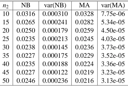
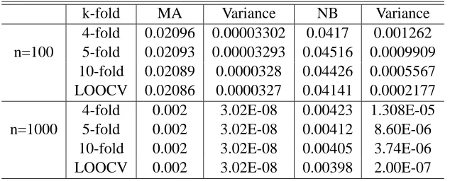
Table 1 presents the results of the simulation. The first column of the table shows the size of the test set. The second column reports the value of the Nadeau and Bengio estimator, while the third column reports its variance. The variance is computed by simply taking the sample variance of the estimator that was computed over the 100 independent data sets. The fourth column of the table reports the value of the moment approximation estimator of the variance of the cross validation estimator of the generalization error, while the fifth column reports the sample variance of the moment approximation estimator.
n2 NB var(NB) MA var(MA)
10 0.0316 0.000310 0.0328 7.75e-06 15 0.0265 0.000241 0.0282 5.34e-05 20 0.0250 0.000179 0.0259 4.50e-05 25 0.0235 0.000213 0.0245 4.03e-05 30 0.0238 0.000145 0.0236 3.73e-05 35 0.0227 0.000175 0.0229 3.52e-05 40 0.0235 0.000188 0.0224 3.36e-05 45 0.0227 0.000122 0.0219 3.23e-05 50 0.0246 0.000236 0.0216 3.13e-05
Table 1: Simple mean case n=100, J=15. Nadeau-Bengio (NB) and moment approximation (MA) estimators of the variance of the cross validation estimator of the generalization error, and their sample variances. J=15, and the results are averages over 100 independent data sets. The size of the data universe is 100.
We notice that the variance of the moment approximation estimator is at least one order of mag-nitude smaller than the variance of the Nadeau- Bengio estimator, thereby increasing the accuracy of the moment estimator.
size of the test set
10 20 30 40 50
0.022
0.024
0.026
0.028
0.030
0.032
nb ma
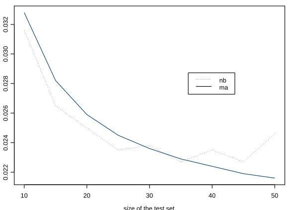
Figure 1: Simple mean case n=100, J=15
seems to fluctuate (this also is indicated by the value of the sample variance associated with the estimator and reported in table 1.)
n2 NB var(NB) MA var(MA)
10 0.0235 1.24e-04 0.0241 7.75e-06 15 0.0212 8.77e-05 0.0227 3.47e-05 20 0.0211 6.27e-05 0.0220 3.26e-05 25 0.0204 7.50e-05 0.0216 3.13e-05 30 0.0206 7.28e-05 0.0213 3.05e-05 35 0.0203 6.79e-05 0.0211 2.98e-05 40 0.0204 7.94e-05 0.0209 2.93e-05 45 0.0213 8.08e-05 0.0207 2.88e-05 50 0.0206 6.43e-05 0.0206 2.84e-05
Table 2 presents the variance estimates of the CV estimators of the generalization error when J=50. In this case we notice that the variance of the moment approximation estimator is about half of the variance of the Nadeau-Bengio estimator.
size of the test set
10 20 30 40 50
0.021
0.022
0.023
0.024
nb ma
Figure 2: Simple mean case n=100, J=50
Figure 2 shows a plot of Nadeau-Bengio and moment approximation estimate of the variance as a function of the size of the test set. The larger variance of the Nadeau-Bengio estimator that was reported in table 2 can also be seen again in Figure 2.
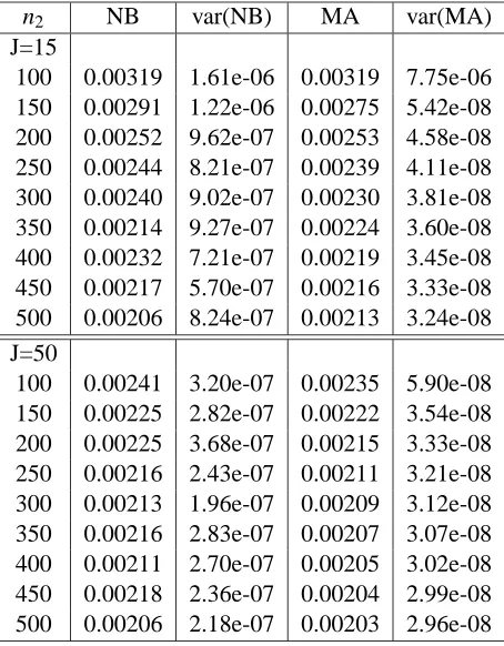
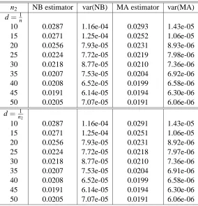
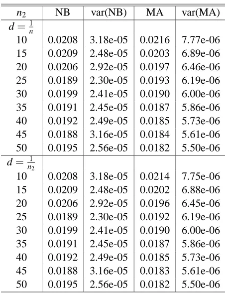
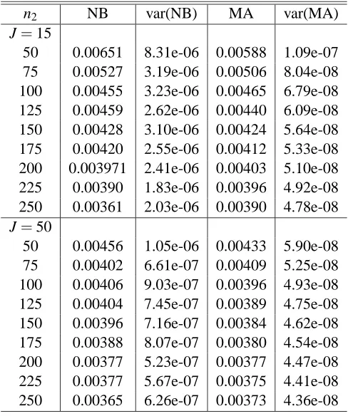
Table 3 presents the values of the two variance estimators as well as their variance when the data universe has size n=1000, for the case J=15 and J=50. We notice that the performance, in terms of variance, of the moment approximation estimator is, in both cases, superior to the performance of the Nadeau-Bengio estimator, always having variance that is smaller than the NB variance by one order of magnitude.
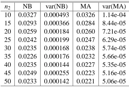
To address the problem of bias we computed the exact (and theoretical) value of the variance estimator ofn2
n1ˆµJ. Therefore, we computed, using formula (3.1), Var(
n2
n1ˆµJ)under square error loss and under the assumption of a N(0,1)distribution. The distributional assumption is used to obtain the theoretical value. This is done only for the purpose of comparison and in order to allow a bias computation to be carried out without having to estimate higher order moments. In practice, the distribution of the population from which the data arise is not known, and higher order moments need to be estimated from the data.
The exact theoretical value of Var(ˆµj)is
Var(ˆµj) =
2 n2{
1+ 2
n1 +n2
n2 1
n2 NB var(NB) MA var(MA)
J=15
100 0.00319 1.61e-06 0.00319 7.75e-06 150 0.00291 1.22e-06 0.00275 5.42e-08 200 0.00252 9.62e-07 0.00253 4.58e-08 250 0.00244 8.21e-07 0.00239 4.11e-08 300 0.00240 9.02e-07 0.00230 3.81e-08 350 0.00214 9.27e-07 0.00224 3.60e-08 400 0.00232 7.21e-07 0.00219 3.45e-08 450 0.00217 5.70e-07 0.00216 3.33e-08 500 0.00206 8.24e-07 0.00213 3.24e-08 J=50
100 0.00241 3.20e-07 0.00235 5.90e-08 150 0.00225 2.82e-07 0.00222 3.54e-08 200 0.00225 3.68e-07 0.00215 3.33e-08 250 0.00216 2.43e-07 0.00211 3.21e-08 300 0.00213 1.96e-07 0.00209 3.12e-08 350 0.00216 2.83e-07 0.00207 3.07e-08 400 0.00211 2.70e-07 0.00205 3.02e-08 450 0.00218 2.36e-07 0.00204 2.99e-08 500 0.00206 2.18e-07 0.00203 2.96e-08
Table 3: Simple mean case n=1000, J=15 and J=50. Moment approximation (MA) and Nadeau-Bengio (NB) estimators of the variance of the cross validation estimator of the generaliza-tion error under random selecgeneraliza-tion, and their sample variances. The size of the data universe is n=1000 and J=15 and 50.
Using theorem 3.1 the approximation to the value of Var(ˆµj)is
Var(ˆµj) =
2 n2{
1+ 2
n1
+O(1
n21)}. The same theorem provides the approximation to Cov(ˆµj,ˆµj0)as follows:
Cov(ˆµj,ˆµj0) =2
n(1+ 2 n) +O(
1 n21).
The exact theoretical computation of the covariance provides us with the formula
Cov(ˆµj,ˆµj0) =2
n(1+ 2 n) +
2 n1
(1
n1−
1 n).
Using these expressions we computed the exact value of the variance ofn2
n2 Exact Variance Bias of MA estimator Bias of NB estimator
10 0.0327 0.0001 -0.0011
15 0.0282 0 -0.0017
20 0.0259 0 -0.0009
25 0.0246 -0.0001 -0.0011
30 0.0237 -0.0001 0.0001
35 0.0232 -0.0003 -0.0005
40 0.0227 -0.0003 0.0008
45 0.0223 -0.0004 0.0004
50 0.0222 -0.0006 0.0024
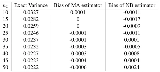
Table 4: Bias of MA and NB estimators. Bias of MA of NB estimators for the case of the simple mean. The data universe has size 100, J=15. The bias is calculated as the expectation of the estimator minus the exact value.
and J=15. We observe that the moment approximation estimator has a very small bias, consistently smaller than the bias of the Nadeau-Bengio estimator. Notice that when the sizes of the training and test sets are equal (n1=n2=50) the bias of the Nadeau-Bengio estimator is four times higher, in
absolute value, than that of the moment approximation estimator.
At this point, we remind the reader that the Nadeau-Bengio estimator given in (2.5) is generally applicable. The proposed estimators take advantage of information about the data and the learning algorithm. Hence, it is not completely surprising that they perform better than the Nadeau Bengio estimator in terms of variance and bias.
For comparison reasons, after a referee’s suggestion, we computed the second estimator pro-posed by Nadeau and Bengio(2003) and given by (2.6). Table 5 presents the values of the estima-tors of the variance given by (2.5) and (2.6) and the moment approximation estimator. Expressions (3.9) and (3.10) were used to obtain the needed variance and covariance terms. The size of the data universe is 50, 100, 500 and 1000, the size of the test set is taken to be 10, 20, 100 and 200 and J is either 15 or 50. ¿From table 5 we see that the estimator given by (2.6) is indeed conservative; its value is almost twice as big as the value of either the cheap to compute Nadeau and Bengio esti-mator given by (2.5) and the moment approximation estiesti-mator. It is interesting to notice that, when the training set size is the same with the training set size used to compute (2.5) and the moment approximation estimator, the value of (2.6) is comparable to the value of the other two estimators. This observation indicates the importance of the size of the training set in the computation of the variance of the cross-validation estimators of the generalization error.