http://dx.doi.org/10.4236/tel.2015.51018
How to cite this paper: Dubé, J. and Legros, D. (2015) Modeling Spatial Data Pooled over Time: Schematic Representation and Monte Carlo Evidences. Theoretical Economics Letters, 5, 132-154. http://dx.doi.org/10.4236/tel.2015.51018
Modeling Spatial Data Pooled over Time:
Schematic Representation and Monte Carlo
Evidences
Jean Dubé1, Diego Legros2 1Laval University, Québec, Canada 2University of Burgundy, Dijon, France
Email: mailto:[email protected], mailto:[email protected]
Received 24 January 2015; accepted 11 February 2015; published 15 February 2015
Copyright © 2015 by authors and Scientific Research Publishing Inc.
This work is licensed under the Creative Commons Attribution International License (CC BY).
http://creativecommons.org/licenses/by/4.0/
Abstract
The spatial autocorrelation issue is now well established, and it is almost impossible to deal with spatial data without considering this reality. In addition, recent developments have been devoted to developing methods that deal with spatial autocorrelation in panel data. However, little effort has been devoted to dealing with spatial data (cross-section) pooled over time. This paper endea-vours to bridge the gap between the theoretical modeling development and the application based on spatial data pooled over time. The paper presents a schematic representation of how spatial links can be expressed, depending on the nature of the variable, when combining the spatial mul-tidirectional relations and temporal unidirectional relations. After that, a Monte Carlo experiment is conducted to establish the impact of applying a usual spatial econometric model to spatial data pooled over time. The results suggest that neglecting the temporal dimension of the data generat-ing process can introduce important biases on autoregressive parameters and thus result in the inaccurate measurement of the indirect and total spatial effect related to the spatial spillover effect.
Keywords
Spatio-Temporal Data, Data Generating Process, Spatial Econometric, Weights Matrices, Monte Carlo Experiment
1. Introduction
133
The particularity of spatial autocorrelation lies in its multidirectional effect. Its complexity explains why spatial autocorrelation has received such attention since spatial data are now widely available and used. Spatial auto- correlation among residuals of a statistical model can have various consequences on estimated coefficients and variances, depending on sample size [3]-[5].
Spatial autocorrelation is also the starting point of the development of spatial econometrics begun at the end of the decade 1970 [6]. The most recent development in the field focuses on spatial panel models and the deve- lopment of an appropriate estimation procedure [7]. Most of the literature now focuses on how it can be possible to take into account the spatial characteristics of the data, while using the temporal source of variability as well. Essentially, these approaches apply very well to data representing given geometric delimitation, such as a region, provinces, states and countries. However, there are many databases that do have both dimensions, spatial and temporal, but are clearly different from the panel case.
Spatial, or cross-sectional, databases pooled over time can represent sale prices (real estate), business opening (or)/closings, crime location, innovation, and so on. For these databases, the panel procedures cannot be applied since a given spatial observation (located at a point) is only observed once1 over time. In short, spatial data collected over time can clearly be different from the spatial panel case. Since panel applications fail to adequately model spatial data pooled over time, the easy solution for researchers is normally to apply the usual spatial econometric methods and models. However, such applications implicitly assume that time dimension has no effect on the data generating process. Even worse, this approach assumes that future observations can influence the determination of past values of the dependent variable [8].
Recent developments have proposed a simple way to adequately control the temporal dimension while accounting for spatial dimension influencing the data generating process [8]-[11] when data consist of spatial obser- vations pooled over time. However, very few have investigated the effect of adopting spatial econometric tech- niques for such data. Thus, there is a real need to determine the exact effect of applying spatial econometric models and spatial autocorrelation detection tests on spatial data pooled over time.
The paper endeavours to determine the impact of using spatial econometric models and tests when data consist of individual spatial units pooled over time. More specifically, the paper presents a realistic representation of the data generating process (DGP) for spatial data pooled over time by decomposing the possible relations for the dependent variable and for the error term. A Monte Carlo experiment formalizes this DGP and investigates the effects of neglecting the temporal dimension when estimating spatial autoregressive models. The results clearly suggest that neglecting the temporal dimension of the DGP can generate biases on the autoregressive coefficient as well as on the coefficient related to the independent variable which can lead to erroneous inter- pretation of the indirect and total marginal effect related to spatial characterization [4].
The paper is divided into five sections. The first section formally addresses the characteristics of spatial data pooled over time through a visual presentation of the DGP. Particular attention is paid to the ties and relationship (unidirectional and multidirectional) that can arise from spatial data pooled over time. The second section presents the way a weights matrix can be adapted and decomposed to deal simultaneously with the spatial and temporal dimensions. The third section presents a simple Monte Carlo framework used to evaluate the impact of neglecting the temporal dimension of the DGP on the estimation of the coefficients as well as on the general Moran’s I [12] index used to detect spatial autocorrelation. The estimation procedure is briefly discussed. The fourth section presents the results and discusses the possible biases of neglecting the temporal dimension. Lastly, the paper concludes with a summary of the main results.
2. Data Generating Process of Spatial Data Pooled over Time
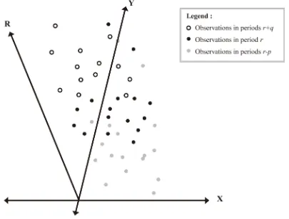
The data generating process of spatial data pooled over time is based on a three dimensional representation: the dimension X representing the east-west location of a given point, the dimension Y representing the north- south location of the point and the dimension R indicating the time period the point was collected (Figure 1). It is no longer based on a two dimensional configuration as is the case for spatial data (Figure 2). The three dimensional representation complicated the application of the usual spatial models and tests [8]. Since an addi- tional dimension is added on the DGP, the relations are not necessarily multidirectional for all observations. In fact, the possible relation among the variables depends on the nature of the variables considered.
134
Figure 1. Schematic representation of the spatio-temporal distribution of the observations.
[image:3.595.97.502.400.708.2]135
tional spatial relations are only possible for a given time period2. Otherwise, it supposes that the future can be perfectly anticipated so that actual realizations of the dependent variable, yir, can influence the realizations of
another dependent variable, but occurring some period before, yj r p(− ). Usual multidirectional links between observations will implicitly assume that future realizations, yj r q( + ), can influence past or actual realizations,
( )
i r p
y − or yir, which is a strong assumption based on the fact that perfect anticipation of future realizations is
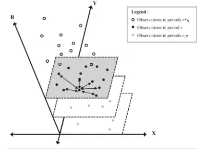
always right. This assumption is particularly criticized when working with a considerable temporal dimension. For this reason, spatial multidirectional relations need to be limited to the same time period, as indicated with the bidirectional arrow, which only occurs between the black points (Figure 3).
Of course, the prior realizations can also influence the actual realizations of the dependent variable. However, the relation is no more multidirectional, but rather unidirectional: the past observations can influence the actual realizations, but the inverse is not possible. The temporal unidirectional constraints of the links can be used to introduce new relations among observations. The unidirectional relations are represented through a unidirec- tional arrow, indicating that the flow of the relations becomes truncated in one direction between the grey points and the black points (Figure 4).
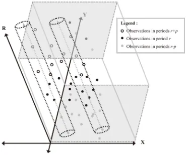
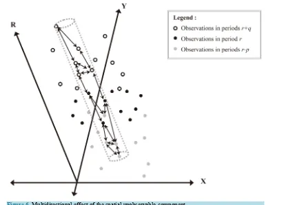
[image:4.595.98.486.386.678.2]Of course, the DGP can also be influenced by some (latent) fixed spatial effects. This component, usually refered to as the omitted variable problem, is usually hidden through the error term. This effect can be multi- directional if the spatial structure is assumed to be constant (and unchanged) over time. The model then assumes that the autoregressive specification is decomposed through the error component [13]. This is the essence of the geo-statistical approaches that assume that latent structure, represented here by the dotted arrow, is constant and present in all time periods, but limited to a delimited or local vicinity (Figure 5). The latent structure leads to multidirectional relations, as expressed by the bidirectional arrows (Figure 6), between observations collected at different time periods.
Figure 3. Schematic representation of the multidirectional spatial effect for a given time period and a particular point.
136
Figure 4. Schematic representation of the unidirectional spatial effect for a given time period and a particular point.
[image:5.595.115.484.397.706.2]137
Figure 6. Multidirectional effect of the spatial unobservable component.
Considering temporal constraints related to spatial links among dependent (and independent) variables as well as full multidirectional relations hidden through latent spatial structure gives a completely different represen- tation of the possible links between observations (points) considering the autoregressive process assumed. To some extend, these restrictions to modeling strategies were previously highlighted by what Legendre (1993) [14] calls the new paradigm of spatial autocorrelation.
This representation of the DGP for spatial data pooled over time underlines the pertinence, as mentioned in the literature, of thinking about how the database structure should be analyzed before doing any mechanical construction of the weights matrix. According to some authors, the weights matrix should be based on a-priori
theoretically-defendable knowledge [15] [16]. This idea is also supported by the work of Pinske and Slade (2010) [17] who suggest that approaches should be developed from an empirical perspective and by McMillen (2010) [18] who stresses that what really matters when working with spatial data is the relative position of the observa- tions.
As can be seen, the DGP of spatial data pooled over time is clearly different from the classic spatial case since relations among the observable variables incorporate constraints on the way one needs to consider the autoregressive process. In short, the DGP for spatial data pooled over time is different from the spatial case, where all relations are multidirectional, and different from the panel case, where individual observations are repeated in each time period. It is then necessary to consider the possible complex schema to make sure that one captures the correct (spatial and temporal) effects.
It is also necessary to develop an adapted notation when data consist of spatial individual units pooled over time. In the spatial case, the total sample is usually denoted by N, while in the spatial panel case, the total sample is denoted by N T× , where N is the number of spatial observations and T is the number of time periods considered. Since the spatial panel case reports the same number of observations in each time period, 1,2, , R, the sum of N over the total time period, T =
∑
Rr=1r time period is simply equal to N T× . How- ever, in the case of spatial data pooled over time, the total number of observations in a given time period r, is noted Nr. The sample size can be different in each time period so that the total sample size is simply given by138
Summarized, the techniques from the spatial panel data case cannot be applied when individual spatial units are not repeated over time. Moreover, the spatial econometric techniques implicitly assume that temporal di- mension has no effect on the DGP, which is a strong and possibly false assumption. However, these techniques may be applied if the weights matrix accounts correctly for possible relations among the individual units. To do so, it is necessary, before turning to the Monte Carlo experiment, to determine the possible form of the weights matrix for spatial data pooled over time. The next section discusses the construction of such weights matrices expressing the multidirectional effect among observations for a given time period as well as the unidirectional relations coming from a previous time period.
3. Building an Appropriate Weights Matrix
The usual spatial weights, sij, among two observations i and j is built using information on the geogra- phical location of both observations, given by the couples
(
X Yi, i)
and(
X Yj, j)
. The distance separating the two points, noted dij, can be calculated using the Pythagorean theorem (Equation (1))3.(
) (
2)
2ij i j i j
d = X −X + Y Y− (1)
Next, a mathematical transformation to these individuals distance is applied to make sure that the final spatial relations, or weights, summarize the idea behind the first law of geography [19]: everything is related to every- thing else, but closer things more so. Without loss of generality, it is possible to cite the three most empirically used transformation function related to distance, dij: i) the inverse, or square inverse, distance function (Equation (2)); ii) the exponential negative function of the distance (Equation (3)); iii) the nearest neighbors function (Equation (4)).
if 0 otherwise
ij ij
ij
d d d
s = −α ≤
(2)
e if 0 otherwise
ij
d ij
ij d d
s = − ≤
(3) 1 if 0 otherwise i ij k ij d d
s = ≤
(4) where α (Equation (2)) is a penalty parameter imposed on distance reflecting the inverse distance transfor- mation
(
α=1)
or the inverse square distance transformation(
α=2)
, d (Equations (2) and (3)) is a critical distance cut-off value limiting the spatial relation to local consideration or surroundings, and dki (Equation (4)) is a critical cut-off distance value for each point i ensuring that each observation has a fix number( )
k of neighbors. Of course, the definition of the weights matrix can be based on a more complex specification, such as the tri-cube transformation [20], or the gaussian transformation [21] or any other transformation drawn from the geographically weighted regression (GWR) approach [22] [23].In the end, the individual spatial weights, sij can be summarized in a square table (or matrix), noted S, that expresses the spatial relations among all observations (Equation (5)).
12 13 1
12 23 2
13 23 3
1 2 3
0 0 0 0 R R R
R R R
N
N
N
N N N
s s s
s s s
s s s
s s s
=
S (5)
139
For the case of spatial data pooled over time, the spatial weights matrix is of dimension NT×NT, and needs
adjustment before proceeding to any statistical test or model estimation since, as previous mentioned, relations are not necessarily multidirectional. This imposes some constraint on the individual spatial weights, sij in the original specification. Considering the fact that spatial relations may be limited to some spatial consideration, as pointed out by the seminal work of Hègerstrand (1970) [24], the unidirectional effect is limited to a given spatial definition.
As pointed out by some authors [8]-[11] [25], the construction of a temporal weights matrix can help to build spatio-temporal weights matrices. However, this decomposition can also be simplified by introducing constraints on the spatial weights matrix through a block diagonal decomposition.
Assuming that the observations are previously chronologically ordered, so that the first lines in the database represent the oldest observations while the last lines represent the newest observations [26], it is possible to isolate the effect of multidirectional spatial effect for the same time period. This decomposition is simply obtained by building T different spatial weights of a smaller dimension, Srr expressing the spatial relations
among the observations collected in period r. By pooling these individual weights matrices on the diagonal of the global weights matrix, S we obtain a particular weights matrix composed of a block diagonal (Equation (6)).
11
22
33
0 0 0
0 0 0
0 0 0
0 0 0 RR
= S S S S S (6)
where each square spatial weights matrix, Srr, is of dimension N Nr× r and represents potential spatial links
among observations collected in the same time period.
Moreover, given the global spatial weights matrix representation (Equation (5)), the chronological order allows to decompose the unidirectional effect through a block triangular (lower and higher) part. The lower part represents the potential effect of past realizations on actual realizations, while the upper part represents the effect of future realizations on actual realizations. Since it is impossible (or at least strongly unlikely) to know with exactitude the future realizations, the upper triangular part can be set to zero. This constraint implies that working with spatial econometric tests and models with spatial data pooled over time assumes that the assumption of per- fection anticipation is true (or likely). This lack of constraint on the weights matrix can potentially lead to a bias in the estimation, as noted by Smith (2009) [11], related to over-connection of the matrix.
By using only the lower triangular block of the original spatial weights matrix (Equation (7)), one can easily synthesizes the unidirectional relations linking the observation i in period r p− to observation j in period
r q+ , synthesis in the matrix W(r q r p+ )( − ).
21
31 32
1 2 3
0 0 0 0
0 0 0
0 0
0
R R R
= W
W W W
W W W
(7)
Each matrix, of dimension Nr q+ ×Nr p− synthesizes the (unidirectional) spatial relations linking previous realizations observed in period r p− to realizations occurring in period r q+ . The final definition of each lower diagonal block of the matrix is also based on the use of an actualization coefficients, noted κ(r q r p+ )( − ),
reflecting the temporal distance separating the realizations (Equations (6) and (8)).
(r q r p+ )( − )=κ(r q r p+ )( − )× (r q r p+ )( − )
W S (8)
where:
(r q r p)( )
(
r q) (
1 r p)
q p1κ + − = =
140 and
(r q r p+ )( − )
S (10)
denotes the lower triangular part of the full weights matrix S. It should be noted, at this stage, that the use of the weights matrix W can introduce a possible problem in the estimation process since it is not of full rank. We will come back to this point later.
Both information can be synthesized through a unique spatio-temporal weights matrix (Equation (11)) by adding the weights matrix for multidirectional spatial effect for a given time period (Equation (6)) to the weights matrix accounting for unidirectional spatial effect based on a previous time period (Equation (7)).
= +
W S W (11) The reader can easily show that this block decomposition leads to the same matrix as using the Hadamard product of a spatial weights matrix and a temporal weights matrix. However, the advantage of treating weights matrices as separate (Equations (6) and (7)) instead of a unique matrix (Equation (11)) is that the effect can be expressed, as in Pace et al. (1998, 2000) [26] [27] as the sum of two distinct component: i) a spatial multidirec- tional effect; and ii) a spatial dynamic unidirectional effect.
Given the choice of the users, the final specifications of the weights matrix can then be row standardized, as is common in empirical applications. The row-standardization procedure is a common practice that ensures the comparability of the usual statistic tests as well as the autoregressive estimated coefficients.
Given the structure of the weights matrix accounting for spatial and temporal dimensions of the DGP, it is now possible to test whether the use of a strictly spatial weights when dealing with spatial data pooled over time introduces bias in the detection tests of spatial autocorrelation and the estimated autoregressive coefficients. To make sure these results can be generalized, a Monte Carlo experiment is conducted.
4. A Monte Carlo Experiment
Given the DGP of the spatial data pooled over time, two general models, based on the different weights matrix specifications developed, can be used to generate data incorporating multidirectional spatial effect for the same time period as well as unidirectional spatial effect occurring from a previous period.
The first model assumes that the true model is given by a linear specification in the parameters (Equation (12)). This DGP can be seen as a given equation based on real indices, as opposed to the nominal indices, where the dependent variable y has the same base value (or definition) for all the time periods.
y yρ yψ Zβ η
η ηλ
= + + +
= +
S W
S (12) where y is the vector of dependent variable of dimension NT×1, Z is a vector of independent variable of dimension NT×1, that can be seen as resulting from a principal component analysis (PCA) summarizing all the pertinent information in a unique variable, η is a vector of spatially dependent error term of dimension NT×1 and is a vector of independent and identically distributed error term of dimension NT×1.
Another specification of the model can be based on a nominal value instead of a real value index. In such a situation, it is common practice to introduce a time trend
( )
t variable (or a matrix of dummy variables for the full time period) to control for temporal heterogeneity and the nominal aspect of the dependent variable [28] (Equation (13)).y yρ yψ tδ Zβ η
η ηλ
= + + + +
= +
S W
S (13) where t is a vector of the trend variable taking a value of 0 in the first period, a value of one in the second period, a value of 2 in the third period and so on. The δ parameter is the coefficient that measures the mean growth rate over the whole sample period.
In both specifications, the weights matrices S, W and S, all of dimension NT×NT are, respectively, a
141
tions collected in the previous time period and a spatial weights matrix controlling for a constant spatial latent component4.
The ρ coefficient represents the usual spatial spillover effect for the actual time period, the ψ coefficient measures the unidirectional spatial effect, which can be seen as a (temporal) dynamic effect spatially located, while the λ coefficient measures the intensity of the spatial autoregressive process related to the error term, which can be seen as an omitted spatial fixed component capturing the latent spatial structure of the DGP. Finally, the β coefficient is the marginal effect of the independent variable on the dependent variable. Given the size of the vectors (or matrix) of variables (dependent and independent), all coefficients are scalars in this framework.
In the model, the variable Wy is known and assumed exogenous since it is based on previous observations. This variable synthesizes the mean outcome of the dependent variable occurring one
(
r−1)
time period prior. These outcomes are, by definition, independent and strictly exogenous from the actual observation since a point is only observed once and the realizations are observed in previous period. However, as previously mentioned, the first N1 lines of this new variable are only composed of elements equal to zero (Equation (11))5 since the elements in the first N1 lines of the weights matrix, W , are all equal to zero.Isolating the dependent variable on the left hand side gives the final expression of the DGP (Equations (14) and (15)) which generates the true value of the dependent variable given the values of the independent variables and the error term.
(
)
1(
(
)
1)
y ρ ψ − Zβ ηλ −
= I S− +W + I S− (14)
(
)
1(
(
)
1)
y ρ ψ − tδ Zβ ηλ −
= I S− +W + + I S− (15)
where I is the identity matrix of dimension NT×NT. Ultimately, the value of y can be obtained if the
geographical coordinates of the individual observations
(
X Yi, i)
are available, if the time period of collection( )
r is known as well as the value of the dependent variable Z and the value of the error terms .For the exercise, the geographical coordinates
(
X Yi, i)
of the observations are simulated assuming that eachcoordinate is distributed from a uniform law (0,10). The temporal dimension variable, r, is constructed from a continuous and intermediate time variable, r, also obtained from a uniform law (0,10). This intermediate variable is then split in ten different discrete time periods: if r varies between 0 and 1, then r=1, if r varies between 1 and 2 then r=2, and so on. These three variables are fundamental to build the spatio-temporal weights matrices, S and W . Finally, it is assumed that the independent variable, Z, is normally distributed with a zero mean and a variance equal to nine (9). The independent error term, is also normally distributed with a zero mean and a homoscedastic unitary variance.
Since the objective of the paper is to explore the effect of neglecting the temporal dimension of the DGP on the autoregressive parameter, the parameter β is set to one, while the parameter δ is set to 0.05. Only the autoregressive parameters, ρ, λ and ψ can vary in the simulations.
4.1. The Estimation Method
Because the model uses a variable based on realizations recorded one period before, Wy it is necessary to assume that the first time period is exogenous in the simulation process. Thus, the observations related to the first time period are not used in the estimation process. Consequently, the model is not estimated using the whole sample size NT, but is, instead, based on NT−1 observations, where 1 2
R
T t t
N − =
∑
=N . In the end, the final sample size is reduced by N1, the total number of observation in the first time period6.This modification is similar to the Cochrane-Orcutt transformation used to estimate a temporal autoregressive model. This procedure is also used when dealing with spatial panel data or panel data. Since it is impossible to 4The spatial weights matrix S could also be replaced by the W matrix as expressed in the Equation (11). However, this exercise has not been considered in the paper.
5This point will be considered in the next section since it introduces a false zero value in the estimation process and potential bias on the es-timation of the ψ coefficient.
6Expressed otherwise, the total sample size can be written as
1 1
T T
142
have information on the initial time period
(
t=0)
, this transformation is necessary to avoid false zero values in the time lag variable for t=1 and introduce potential bias on the ψ parameter. Thus, the vectors of variable are now of dimension NT−1×1 and the weights matrices are of dimension NT−1×NT−1.For the subsequent time period
(
t=2, , R)
, the model can be estimated using the maximum likelihood procedure [29]. However, this procedure can have some minor effect on the precision of the estimation of the parameter λ since some observations can be dropped from the full nearest neighbors matrix. However, the subtraction of about one-ten of the full sample should not be overly significant.4.2. The Values of the Parameters
The results are based on 1000 simulations of 1000 observations
(
NT =1,000)
for the endogenous variable y for the two GDP (12) and (13) and imply different values of the parameters λ, ρ and ψ. The values of the parameter λ and ρ are set to 0.1; 0.3; 0.5 and 0.7, while the parameter ψ can take values of 0.1; 0.2; and 0.3. These values are in line with what previous study found to be the estimated values of the dynamic spatially located dependent variable [8] [9] [30] [31], while it ensure that the sum of the autoregressive parameter on the dependent variable is still lower then one(
ρ ψ+ ≤1)
.For the DGP, the weights matrices are chosen as follows:
the spatial weights matrix, S, is based on the ten (10) nearest neighbors,the matrix;
the spatial weights matrix accounting for multidirectional spatial effect of the dependent variable, S, is based on a negative exponential transformation of the distances separating all observations i and j occurring in the same time period t;
the spatial weights matrix accounting for unidirectional (dynamic) spatial effect of the dependent variable,
W , is also based on a negative exponential transformation of the distances separating an observation i
collected in time period t−1 and another observation j occurring in the next time period t.
It should be noted that both spatio-temporal weights matrices, S and W , are constructed using a general spatial weights matrix and using the block diagonal decomposition (see the previous section). Thereafter, the different models (Equations (12) and (13)) are estimated assuming that: i) the usual spatial econometric model is used and no time lag variable is introduced7; and ii) the model is estimated using the spatio-temporal con- siderations of the DGP.
5. Results
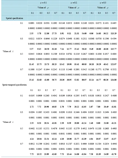
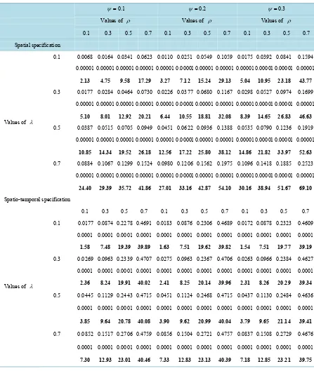
The first conclusion is related to the use of the Moran’s I index8. For low values of ρ and λ, the results clearly suggest that these statistics are not biased toward rejection of the null hypothesis of absence of spatial autocorrelation, as previously proposed by Dubé and Legros (2013) [9]. In fact, when all the autoregressive coefficients are low, including the parameter ψ, the index estimated is lower using a spatial weights matrix instead of the spatio-temporal weights matrix (Table 1 and Table 2). However, the estimated variance of the Moran’s I is also lower. In fact, the lower estimate variance has an important effect for high values of ρ, λ and ψ. In this context, the low variance has an important incidence on the over estimation of the Moran's I
statistic towards systematic rejection of the null hypothesis. This is where the findings of [9] really apply. The conclusions are identical given the specification used (Equations (12) and (13)).
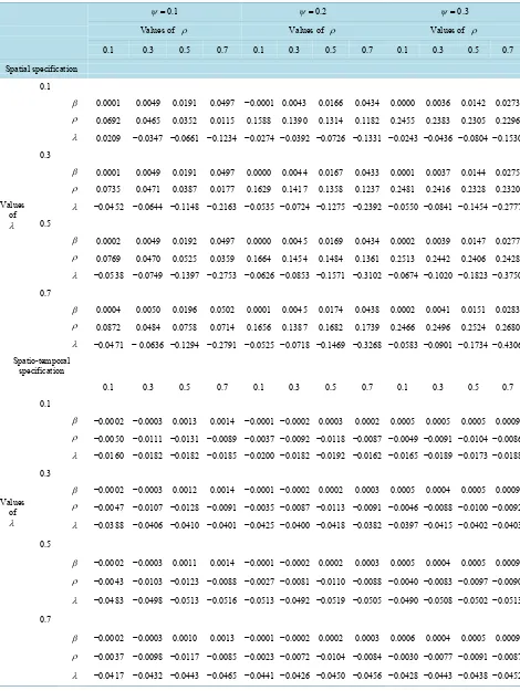
Turning our attention to the coefficients, the effect of spatial specification in a spatio-temporal context can be analyzed through the usual statistics such as the bias, which is defined as Eθ θˆ− , where θ is the real value of the parameter of interest and ˆθ is the estimation of the parameter θ obtained with the Monte Carlo simu- lations, and the mean square error (MSE), defined as E
( )
θ θˆ− 2 . The first statistic allows to compare the capability of the model to return the right answer, while the MSE allows to measure the precision of the estima- tion.
7The variable Wy is not used and the S weights matrix is replaced by the usual full spatial weights matrix, S.
8The formula for the Moran's index is: I e We
e e
′ =
143
Table 1. Synthesis of results for the Moran’s I index (Model 1).
0.1
ψ = ψ =0.2 ψ =0.3
Values of ρ Values of ρ Values of ρ
0.1 0.3 0.5 0.7 0.1 0.3 0.5 0.7 0.1 0.3 0.5 0.7
Spatial specification
Values of λ
0.1 0.0091 0.0220 0.0501 0.1092 0.0146 0.0353 0.0838 0.2163 0.0231 0.0572 0.1431 0.4495
0.00002 0.00002 0.00002 0.00002 0.00002 0.00002 0.00002 0.00002 0.00002 0.00002 0.00002 0.00002
2.55 5.78 12.86 27.73 3.91 9.11 21.31 54.60 6.06 14.63 36.22 113.29
0.3 0.0212 0.0354 0.0646 0.1229 0.0274 0.0498 0.1001 0.2311 0.0368 0.0730 0.1596 0.4594
0.00002 0.00002 0.00002 0.00002 0.00002 0.00002 0.00002 0.00002 0.00002 0.00002 0.00002 0.00002
5.57 9.15 16.50 31.18 7.14 12.77 25.42 58.33 9.49 18.60 40.36 115.77
0.5 0.0445 0.0616 0.0933 0.1509 0.0524 0.0782 0.1319 0.2617 0.0633 0.1036 0.1917 0.4804
0.00002 0.00002 0.00002 0.00002 0.00002 0.00002 0.00002 0.00002 0.00002 0.00002 0.00002 0.00002
11.45 15.75 23.73 38.23 13.42 19.90 33.41 66.03 16.18 26.29 48.42 121.07
0.7 0.1000 0.1247 0.1644 0.2245 0.1118 0.1460 0.2091 0.3415 0.1268 0.1771 0.2706 0.5352
0.00002 0.00002 0.00002 0.00002 0.00002 0.00002 0.00002 0.00002 0.00002 0.00002 0.00002 0.00002
25.42 31.63 41.60 56.75 28.36 36.95 52.82 86.07 32.14 44.77 68.26 134.86
Spatio-temporal specification
Values of λ
0.1 0.3 0.5 0.7 0.1 0.3 0.5 0.7 0.1 0.3 0.5 0.7
0.1 0.0195 0.0909 0.2363 0.4842 0.0199 0.0916 0.2395 0.4871 0.0188 0.0918 0.2427 0.4860
0.0001 0.0001 0.0001 0.0001 0.0001 0.0001 0.0001 0.0001 0.0001 0.0001 0.0001 0.0001
1.72 7.72 19.96 40.85 1.76 7.79 20.22 41.05 1.67 7.80 20.49 41.01
0.3 0.0294 0.1005 0.2433 0.4861 0.0298 0.1010 0.2464 0.4894 0.0285 0.1013 0.2494 0.4883
0.0001 0.0001 0.0001 0.0001 0.0001 0.0001 0.0001 0.0001 0.0001 0.0001 0.0001 0.0001
2.55 8.53 20.54 41.01 2.59 8.59 20.80 41.24 2.48 8.60 21.06 41.21
0.5 0.0482 0.1185 0.2551 0.4876 0.0485 0.1185 0.2579 0.4912 0.0470 0.1188 0.2603 0.4903
0.0001 0.0001 0.0001 0.0001 0.0001 0.0001 0.0001 0.0001 0.0001 0.0001 0.0001 0.0001
4.14 10.04 21.54 41.14 4.16 10.06 21.77 41.39 4.04 10.07 21.97 41.37
0.7 0.0912 0.1599 0.2842 0.4935 0.0910 0.1587 0.2851 0.4964 0.0889 0.1584 0.2854 0.4948
0.0001 0.0001 0.0001 0.0001 0.0001 0.0001 0.0001 0.0001 0.0001 0.0001 0.0001 0.0001
7.75 13.52 23.99 41.63 7.73 13.44 24.06 41.84 7.56 13.39 24.09 41.76
144
Table 2. Synthesis of results for the Moran’s I index (Model 2).
0.1
ψ = ψ =0.2 ψ =0.3
Values of ρ Values of ρ Values of ρ
0.1 0.3 0.5 0.7 0.1 0.3 0.5 0.7 0.1 0.3 0.5 0.7 Spatial specification
Values of λ
0.1 0.0068 0.0164 0.0341 0.0623 0.0110 0.0251 0.0549 0.1059 0.0175 0.0392 0.0841 0.1594 0.00001 0.00001 0.00001 0.00001 0.00001 0.00001 0.00001 0.00001 0.00001 0.00001 0.00001 0.00001
2.13 4.75 9.58 17.29 3.27 7.12 15.24 29.13 5.04 10.95 23.18 43.77
0.3 0.0177 0.0284 0.0464 0.0730 0.0226 0.0377 0.0680 0.1167 0.0298 0.0527 0.0974 0.1699 0.00001 0.00001 0.00001 0.00001 0.00001 0.00001 0.00001 0.00001 0.00001 0.00001 0.00001 0.00001
5.10 8.01 12.92 20.21 6.44 10.55 18.81 32.08 8.39 14.65 26.83 46.63
0.5 0.0387 0.0515 0.0705 0.0949 0.0451 0.0622 0.0936 0.1388 0.0535 0.0790 0.1236 0.1919 0.00001 0.00001 0.00001 0.00001 0.00001 0.00001 0.00001 0.00001 0.00001 0.00001 0.00001 0.00001
10.85 14.34 19.52 26.18 12.56 17.22 25.80 38.12 14.86 21.82 33.97 52.63
0.7 0.0884 0.1067 0.1299 0.1524 0.0980 0.1206 0.1562 0.1975 0.1096 0.1418 0.1885 0.2523 0.00001 0.00001 0.00001 0.00001 0.00001 0.00001 0.00001 0.00001 0.00001 0.00001 0.00001 0.00001
24.40 29.39 35.72 41.86 27.01 33.16 42.87 54.10 30.16 38.94 51.67 69.10
Spatio-temporal specification
Values of λ
0.1 0.3 0.5 0.7 0.1 0.3 0.5 0.7 0.1 0.3 0.5 0.7 0.1 0.0177 0.0874 0.2278 0.4691 0.0183 0.0876 0.2306 0.4689 0.0172 0.0878 0.2323 0.4609
0.0001 0.0001 0.0001 0.0001 0.0001 0.0001 0.0001 0.0001 0.0001 0.0001 0.0001 0.0001
1.58 7.48 19.39 39.89 1.63 7.51 19.62 39.82 1.54 7.51 19.77 39.19
0.3 0.0269 0.0963 0.2339 0.4707 0.0275 0.0963 0.2367 0.4706 0.0263 0.0966 0.2384 0.4627 0.0001 0.0001 0.0001 0.0001 0.0001 0.0001 0.0001 0.0001 0.0001 0.0001 0.0001 0.0001
2.36 8.24 19.91 40.02 2.41 8.25 20.14 39.96 2.31 8.26 20.29 39.34
0.5 0.0445 0.1129 0.2443 0.4715 0.0451 0.1124 0.2468 0.4715 0.0437 0.1130 0.2484 0.4636
0.0001 0.0001 0.0001 0.0001 0.0001 0.0001 0.0001 0.0001 0.0001 0.0001 0.0001 0.0001
3.85 9.64 20.78 40.08 3.90 9.62 20.99 40.04 3.79 9.65 21.14 39.41
0.7 0.0852 0.1517 0.2706 0.4759 0.0856 0.1504 0.2721 0.4757 0.0837 0.1508 0.2729 0.4676
0.0001 0.0001 0.0001 0.0001 0.0001 0.0001 0.0001 0.0001 0.0001 0.0001 0.0001 0.0001
7.30 12.93 23.01 40.46 7.33 12.83 23.13 40.39 7.18 12.85 23.21 39.75
145
Table 3. Synthesis of the bias on the parameter-spatial vs. spatio-temporal consideration (Model 1).
0.1
ψ = ψ =0.2 ψ =0.3
Values of ρ Values of ρ Values of ρ
0.1 0.3 0.5 0.7 0.1 0.3 0.5 0.7 0.1 0.3 0.5 0.7 Spatial specification
Values of λ
0.1
β 0.0001 0.0049 0.0191 0.0497 −0.0001 0.0043 0.0166 0.0434 0.0000 0.0036 0.0142 0.0273
ρ 0.0692 0.0465 0.0352 0.0115 0.1588 0.1390 0.1314 0.1182 0.2455 0.2383 0.2305 0.2296
λ 0.0209 −0.0347 −0.0661 −0.1234 −0.0274 −0.0392 −0.0726 −0.1331 −0.0243 −0.0436 −0.0804 −0.1530 0.3
β 0.0001 0.0049 0.0191 0.0497 0.0000 0.0044 0.0167 0.0433 0.0001 0.0037 0.0144 0.0275 ρ 0.0735 0.0471 0.0387 0.0177 0.1629 0.1417 0.1358 0.1237 0.2481 0.2416 0.2328 0.2320
λ −0.0452 −0.0644 −0.1148 −0.2163 −0.0535 −0.0724 −0.1275 −0.2392 −0.0550 −0.0841 −0.1454 −0.2777 0.5
β 0.0002 0.0049 0.0192 0.0497 0.0000 0.0045 0.0169 0.0434 0.0002 0.0039 0.0147 0.0277
ρ 0.0769 0.0470 0.0525 0.0359 0.1664 0.1454 0.1484 0.1361 0.2513 0.2442 0.2406 0.2428
λ −0.0538 −0.0749 −0.1397 −0.2753 −0.0626 −0.0853 −0.1571 −0.3102 −0.0674 −0.1020 −0.1823 −0.3750 0.7
β 0.0004 0.0050 0.0196 0.0502 0.0001 0.0045 0.0174 0.0438 0.0002 0.0041 0.0151 0.0283 ρ 0.0872 0.0484 0.0758 0.0714 0.1656 0.1387 0.1682 0.1739 0.2466 0.2496 0.2524 0.2680
λ −0.0471 − 0.0636 −0.1294 −0.2791 −0.0525 −0.0718 −0.1469 −0.3268 −0.0583 −0.0901 −0.1734 −0.4306 Spatio-temporal
specification
Values of λ
0.1 0.3 0.5 0.7 0.1 0.3 0.5 0.7 0.1 0.3 0.5 0.7 0.1
β −0.0002 −0.0003 0.0013 0.0014 −0.0001 −0.0002 0.0003 0.0002 0.0005 0.0005 0.0005 0.0009 ρ −0.0050 −0.0111 −0.0131 −0.0089 −0.0037 −0.0092 −0.0118 −0.0087 −0.0049 −0.0091 −0.0104 −0.0086
λ −0.0160 −0.0182 −0.0182 −0.0185 −0.0200 −0.0182 −0.0192 −0.0162 −0.0165 −0.0189 −0.0173 −0.0188 0.3
β −0.0002 −0.0003 0.0012 0.0014 −0.0001 −0.0002 0.0002 0.0003 0.0005 0.0004 0.0005 0.0009 ρ −0.0047 −0.0107 −0.0128 −0.0091 −0.0035 −0.0087 −0.0113 −0.0091 −0.0046 −0.0088 −0.0100 −0.0092
λ −0.0388 −0.0406 −0.0410 −0.0401 −0.0425 −0.0400 −0.0418 −0.0382 −0.0397 −0.0415 −0.0402 −0.0403
0.5
β −0.0002 −0.0003 0.0011 0.0014 −0.0001 −0.0002 0.0002 0.0003 0.0005 0.0004 0.0005 0.0009
ρ −0.0043 −0.0103 −0.0123 −0.0088 −0.0027 −0.0081 −0.0110 −0.0088 −0.0040 −0.0083 −0.0097 −0.0090
λ −0.0483 −0.0498 −0.0513 −0.0516 −0.0513 −0.0492 −0.0519 −0.0505 −0.0490 −0.0508 −0.0502 −0.0513
0.7
β −0.0002 −0.0003 0.0010 0.0013 −0.0001 −0.0002 0.0002 0.0003 0.0006 0.0004 0.0005 0.0009
ρ −0.0037 −0.0098 −0.0117 −0.0085 −0.0023 −0.0072 −0.0104 −0.0084 −0.0030 −0.0077 −0.0091 −0.0087
146
Table 4. Synthesis of the bias on the parameter-spatial vs. spatio-temporal consideration (Model 2).
0.1
ψ = ψ =0.2 ψ =0.3
Values of ρ Values of ρ Values of ρ
0.1 0.3 0.5 0.7 0.1 0.3 0.5 0.7 0.1 0.3 0.5 0.7 Spatial specification
Values of λ
0.1
β −0.0002 0.0043 0.0173 0.0399 −0.0005 0.0033 0.0126 0.0224 −0.0006 0.0015 0.0049 −0.0097 δ 0.0061 0.0179 0.0437 0.1529 0.0099 0.0261 0.0763 0.3393 0.0159 0.0436 0.1368 0.8963
ρ 0.0133 −0.0749 −0.2189 −0.6768 0.0665 −0.0424 −0.2913 −1.1946 0.1162 −0.0563 −0.5128 −2.1954
λ −0.0148 −0.0084 0.0104 0.0938 −0.0114 0.0079 0.0749 0.2567 0.0033 0.0477 0.1788 0.4917 0.3
β −0.0005 0.0035 0.0159 0.0378 −0.0010 0.0022 0.0110 0.0201 −0.0014 0.0000 0.0029 −0.0112
δ 0.0069 0.0206 0.0483 0.1580 0.0116 0.0299 0.0827 0.3434 0.0187 0.0495 0.1444 0.8982
ρ 0.0087 −0.0919 −0.2420 −0.7159 0.0557 −0.0659 −0.3230 −1.2545 0.0982 −0.0921 −0.5570 −2.2231
λ −0.0377 −0.0357 −0.0378 −0.0076 −0.0352 −0.0227 0.0137 0.1265 −0.0251 0.0077 0.0948 0.3267 0.5
β −0.0007 0.0027 0.0143 0.0345 −0.0016 0.0011 0.0090 0.0174 −0.0021 −0.0012 0.0007 −0.0103 δ 0.0079 0.0238 0.0537 0.1628 0.0139 0.0346 0.0900 0.3480 0.0221 0.0563 0.1515 0.9014
ρ 0.0103 −0.1047 −0.2711 −0.8103 0.0476 −0.0871 −0.3572 −1.3120 0.0872 −0.1051 −0.6083 −2.1047
λ −0.0476 −0.0479 −0.0651 −0.0816 −0.0452 −0.0382 −0.0280 0.0197 −0.0391 −0.0192 0.0267 0.1745 0.7
β −0.0007 0.0022 0.0136 0.0334 −0.0017 0.0006 0.0081 0.0160 −0.0024 −0.0019 0.0007 −0.0078 δ 0.0091 0.0275 0.0596 0.1681 0.0167 0.0398 0.0976 0.3535 0.0262 0.0634 0.1586 0.9027
ρ 0.0228 −0.1028 −0.2514 −0.7708 0.0631 −0.0761 −0.3349 −1.2789 0.1008 −0.0888 −0.5344 −1.8643
λ −0.0432 −0.0447 −0.0698 −0.1173 −0.0411 −0.0392 −0.0487 −0.0515 −0.0388 −0.0312 −0.0205 0.0387 Spatio-temporal
specification
Values of λ
0.1 0.3 0.5 0.7 0.1 0.3 0.5 0.7 0.1 0.3 0.5 0.7 0.1
β −0.0003 −0.0003 0.0013 0.0015 −0.0001 −0.0002 0.0003 0.0003 0.0005 0.0005 0.0006 0.0010 δ 0.0007 0.0014 0.0014 0.0021 0.0006 0.0012 0.0021 0.0034 0.0010 0.0018 0.0019 0.0073
ρ −0.0069 −0.0127 −0.0153 −0.0102 −0.0055 −0.0112 −0.0139 −0.0108 −0.0066 −0.0109 −0.0124 −0.0115
λ −0.0198 −0.0217 −0.0219 −0.0217 −0.0236 −0.0216 −0.0229 −0.0189 −0.0198 −0.0222 −0.0203 −0.0205 0.3
β −0.0003 −0.0003 0.0012 0.0015 −0.0002 −0.0002 0.0003 0.0003 0.0005 0.0004 0.0005 0.0010 δ 0.0007 0.0014 0.0013 0.0022 0.0005 0.0010 0.0020 0.0036 0.0009 0.0018 0.0018 0.0079
ρ −0.0065 −0.0123 −0.0148 −0.0107 −0.0051 −0.0109 −0.0135 −0.0112 −0.0059 −0.0107 −0.0123 −0.0121
λ −0.0423 −0.0437 −0.0437 −0.0423 −0.0457 −0.0433 −0.0449 −0.0404 −0.0426 −0.0442 −0.0424 −0.0418 0.5
β −0.0003 −0.0003 0.0011 0.0014 −0.0002 −0.0002 0.0002 0.0003 0.0005 0.0004 0.0005 0.0010
δ 0.0005 0.0013 0.0011 0.0021 0.0004 0.0008 0.0019 0.0037 0.0008 0.0017 0.0016 0.0088
ρ −0.0059 −0.0120 −0.0145 −0.0103 −0.0046 −0.0102 −0.0130 −0.0110 −0.0055 −0.0102 −0.0120 −0.0124
λ −0.0509 −0.0521 −0.0538 −0.0532 −0.0535 −0.0516 −0.0543 −0.0520 −0.0512 −0.0528 −0.0518 −0.0526 0.7
β −0.0003 −0.0003 0.0011 0.0014 −0.0002 −0.0002 0.0002 0.0003 0.0005 0.0004 0.0004 0.0009 δ 0.0003 0.0013 0.0009 0.0021 0.0004 0.0005 0.0017 0.0040 0.0006 0.0018 0.0015 0.0103
ρ −0.0054 −0.0115 −0.0136 −0.0100 −0.0039 −0.0095 −0.0125 −0.0108 −0.0046 −0.0100 −0.0115 −0.0121
147
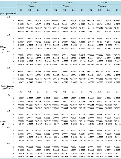
Secondly, the MSE follows a pattern similar to the one of the bias (Table 5 and Table 6). The MSE is comparable within the spatial and spatio-temporal specifications with low values of ρ, λ and ψ , while it clearly becomes larger for spatial specifications for higher values of the autoregressive parameters.
There is a simple way to visualize this conclusion: building a graph of the estimated values of the parameters in each simulation according to the specification selected. Conducting this analysis reinforces the conclusions drawn before (Figures 7-10). First, there is a clear bias in the estimated β coefficient for the specification without trend (Equation (12)), even more for low values of ψ (Figure 7-left panel). For the higher value of ψ, the bias is insignificant, but the precision is clearly affected. For the model introducing a trend, the conclusion is somewhat different: there is no clear bias in the estimated β coefficient, but the estimation of the parameter is clearly imprecise for high values of the autoregressive coefficients.
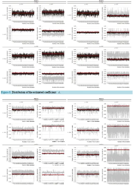
As regards the λ coefficient, the parameter is unbiased with low values of the autoregressive parameters (ρ , λ and ψ ), and this, for both specifications (Figure 8). For high values of ρ in the specification without trend (Equation (12)), the estimation of λ is clearly downward biased. Moreover, the estimation of the parameter is quite imprecise, as shown by the important variation of the grey line. Once again, the conclusion is different considering the specification with a trend (Equation (13)): except for the case of high values of ρ and ψ, there is no evidence of bias in the estimation of λ. However, for high values of the autoregressive coefficient, the imprecision of the estimation is clear.
[image:16.595.63.539.375.706.2]For the ρ coefficient, imprecision is noted in all scenarios (Figure 9). An important bias emerges with larger values of ψ. In fact, the spatial specification is not able to distinguish between the spatial multidirectional effect, as measured by the ρ coefficient in (12) or (13), and the unidirectional spatial effect, measured by ψ. Thus, the important bias comes from the addition of both effect in the unique ρ coefficient in the strictly spatial specification. Moreover, as long as the values of the autoregressive coefficients increase, the imprecision increase. The worst case is noted in the specification (13) with high values of ρ and ψ : in both cases, the
148
[image:17.595.90.517.393.702.2]Figure 8. Distribution of the estimated coefficient λ.
149
Table 5. Synthesis of the mean square error (MSE) on the parameter-spatial vs spatio-temporal consideration (Model 1).
0.1
ψ = ψ =0.2 ψ =0.3
Values of ρ Values of ρ Values of ρ
0.1 0.3 0.5 0.7 0.1 0.3 0.5 0.7 0.1 0.3 0.5 0.7 Spatial specification
Values of λ
0.1
β 0.0001 0.0002 0.0006 0.0029 0.0001 0.0002 0.0005 0.0023 0.0001 0.0002 0.0004 0.0012
ρ 0.0211 0.0148 0.0100 0.0083 0.0414 0.0307 0.0260 0.0209 0.0746 0.0670 0.0603 0.0569
λ 0.0050 0.0064 0.0096 0.0204 0.0055 0.0061 0.0102 0.0230 0.0053 0.0066 0.0114 0.0297
0.3
β 0.0001 0.0002 0.0006 0.0029 0.0001 0.0002 0.0005 0.0023 0.0001 0.0002 0.0004 0.0012
ρ 0.0284 0.0207 0.0148 0.0098 0.0493 0.0361 0.0299 0.0233 0.0813 0.0725 0.0636 0.0586
λ 0.0059 0.0087 0.0181 0.0524 0.0070 0.0092 0.0208 0.0629 0.0071 0.0113 0.0258 0.0844 0.5
β 0.0001 0.0002 0.0006 0.0029 0.0001 0.0002 0.0005 0.0023 0.0001 0.0002 0.0004 0.0013 ρ 0.0404 0.0332 0.0228 0.0127 0.0627 0.0469 0.0389 0.0309 0.0937 0.0859 0.0720 0.0647
λ 0.0061 0.0097 0.0239 0.0813 0.0075 0.0110 0.0288 0.1029 0.0082 0.0143 0.0380 0.1504 0.7
β 0.0001 0.0002 0.0006 0.0029 0.0001 0.0002 0.0005 0.0024 0.0001 0.0002 0.0005 0.0014
ρ 0.0637 0.0547 0.0440 0.0296 0.0845 0.0701 0.0596 0.0485 0.1200 0.1099 0.0942 0.0814
λ 0.0045 0.0073 0.0206 0.0848 0.0056 0.0083 0.0257 0.1147 0.0063 0.0119 0.0354 0.2012 Spatio-temporal
specification
Values of λ
0.1 0.3 0.5 0.7 0.1 0.3 0.5 0.7 0.1 0.3 0.5 0.7 0.1
β 0.0001 0.0001 0.0001 0.0001 0.0001 0.0001 0.0001 0.0001 0.0001 0.0001 0.0001 0.0001
ρ 0.0016 0.0013 0.0010 0.0005 0.0015 0.0012 0.0009 0.0006 0.0014 0.0012 0.0009 0.0005
λ 0.0044 0.0050 0.0053 0.0050 0.0048 0.0046 0.0048 0.0048 0.0046 0.0045 0.0045 0.0052 0.3
β 0.0001 0.0001 0.0001 0.0001 0.0001 0.0001 0.0001 0.0001 0.0001 0.0001 0.0001 0.0001
ρ 0.0016 0.0013 0.0010 0.0005 0.0016 0.0012 0.0009 0.0006 0.0015 0.0012 0.0009 0.0005
λ 0.0049 0.0054 0.0055 0.0052 0.0054 0.0050 0.0052 0.0049 0.0052 0.0051 0.0049 0.0054 0.5
β 0.0001 0.0001 0.0001 0.0001 0.0001 0.0001 0.0001 0.0001 0.0001 0.0001 0.0001 0.0001 ρ 0.0017 0.0013 0.0010 0.0005 0.0016 0.0012 0.0009 0.0006 0.0015 0.0012 0.0009 0.0005
λ 0.0049 0.0052 0.0055 0.0053 0.0053 0.0050 0.0053 0.0051 0.0051 0.0051 0.0050 0.0054 0.7
β 0.0001 0.0001 0.0001 0.0001 0.0001 0.0001 0.0001 0.0001 0.0001 0.0001 0.0001 0.0001 ρ 0.0016 0.0013 0.0010 0.0005 0.0016 0.0011 0.0009 0.0006 0.0014 0.0012 0.0009 0.0005
150
Table 6. Synthesis of the mean square error (MSE) on the parameter-spatial vs spatio-temporal consideration (Model 2).
0.1
ψ = ψ =0.2 ψ =0.3
Values of ρ Values of ρ Values of ρ
0.1 0.3 0.5 0.7 0.1 0.3 0.5 0.7 0.1 0.3 0.5 0.7 Spatial specification
Values of λ
0.1
β 0.0001 0.0002 0.0006 0.0029 0.0001 0.0002 0.0005 0.0032 0.0001 0.0002 0.0009 0.0056 δ 0.0001 0.0006 0.0035 0.0388 0.0003 0.0013 0.0098 0.1616 0.0005 0.0033 0.0294 0.9697
ρ 0.0180 0.0319 0.3231 3.1106 0.0256 0.0457 0.5569 8.0357 0.0411 0.2543 2.3620 19.0776
λ 0.0049 0.0061 0.0124 0.0573 0.0053 0.0074 0.0322 0.1428 0.0055 0.0166 0.0834 0.2982 0.3
β 0.0001 0.0002 0.0005 0.0028 0.0001 0.0002 0.0005 0.0032 0.0001 0.0002 0.0009 0.0055
δ 0.0002 0.0008 0.0042 0.0411 0.0003 0.0017 0.0112 0.1645 0.0007 0.0042 0.0318 0.9810
ρ 0.0230 0.0430 0.3295 3.4607 0.0308 0.0600 0.6025 8.6104 0.0454 0.3470 2.4371 19.0680
λ 0.0054 0.0065 0.0122 0.0416 0.0057 0.0069 0.0214 0.0792 0.0055 0.0123 0.0476 0.1546
0.5
β 0.0001 0.0002 0.0005 0.0030 0.0001 0.0002 0.0005 0.0034 0.0001 0.0002 0.0011 0.0049 δ 0.0002 0.0011 0.0051 0.0433 0.0005 0.0022 0.0130 0.1685 0.0010 0.0052 0.0343 1.0074
ρ 0.0304 0.0567 0.4881 4.6473 0.0400 0.0781 0.8350 9.4234 0.0540 0.2117 3.0228 17.1344
λ 0.0053 0.0065 0.0130 0.0402 0.0057 0.0065 0.0160 0.0475 0.0053 0.0090 0.0261 0.0681 0.7
β 0.0002 0.0002 0.0005 0.0028 0.0001 0.0002 0.0005 0.0031 0.0001 0.0002 0.0010 0.0041
δ 0.0003 0.0014 0.0063 0.0467 0.0006 0.0028 0.0151 0.1760 0.0013 0.0064 0.0374 1.0939
ρ 0.0981 0.1974 0.4734 4.2111 0.0542 0.0969 0.9156 8.8190 0.0677 0.3091 2.5794 14.0381
λ 0.0039 0.0048 0.0101 0.0356 0.0040 0.0046 0.0107 0.0320 0.0039 0.0057 0.0129 0.0300 Spatio-temporal
specification
Values of λ
0.1 0.3 0.5 0.7 0.1 0.3 0.5 0.7 0.1 0.3 0.5 0.7 0.1
β 0.0001 0.0001 0.0001 0.0001 0.0001 0.0001 0.0001 0.0001 0.0001 0.0001 0.0001 0.0001
δ 0.0001 0.0001 0.0001 0.0001 0.0000 0.0001 0.0001 0.0001 0.0001 0.0001 0.0001 0.0003
ρ 0.0016 0.0014 0.0011 0.0006 0.0016 0.0013 0.0010 0.0007 0.0015 0.0012 0.0010 0.0006
λ 0.0046 0.0051 0.0055 0.0052 0.0050 0.0048 0.0050 0.0050 0.0048 0.0048 0.0047 0.0053
0.3
β 0.0001 0.0001 0.0001 0.0001 0.0001 0.0001 0.0001 0.0001 0.0001 0.0001 0.0001 0.0001 δ 0.0001 0.0001 0.0001 0.0001 0.0001 0.0001 0.0001 0.0002 0.0001 0.0001 0.0001 0.0004
ρ 0.0017 0.0014 0.0011 0.0006 0.0016 0.0013 0.0010 0.0007 0.0015 0.0013 0.0010 0.0006
151
Continued
0.5
β 0.0001 0.0001 0.0001 0.0001 0.0001 0.0001 0.0001 0.0001 0.0001 0.0001 0.0001 0.0001
δ 0.0001 0.0001 0.0001 0.0001 0.0001 0.0001 0.0001 0.0002 0.0001 0.0001 0.0001 0.0005
ρ 0.0017 0.0014 0.0011 0.0006 0.0016 0.0013 0.0010 0.0007 0.0015 0.0013 0.0010 0.0006
λ 0.0052 0.0055 0.0058 0.0055 0.0056 0.0053 0.0056 0.0053 0.0053 0.0054 0.0052 0.0056
0.7
β 0.0001 0.0001 0.0001 0.0001 0.0001 0.0001 0.0001 0.0001 0.0001 0.0001 0.0001 0.0001 δ 0.0001 0.0001 0.0002 0.0002 0.0001 0.0002 0.0002 0.0003 0.0001 0.0002 0.0002 0.0007
ρ 0.0017 0.0014 0.0011 0.0006 0.0016 0.0012 0.0010 0.0007 0.0015 0.0012 0.0010 0.0006
[image:20.595.63.541.89.461.2]λ 0.0034 0.0036 0.0037 0.0038 0.0037 0.0034 0.0037 0.0037 0.0035 0.0036 0.0035 0.0037
Figure 10. Distribution of the estimated coefficient δ.
estimation of the coefficient is highly volatile and imprecise.
Finally, turning our attention to the model introducing a trend (Equation (13)), it can be explained why there is no overestimation of the ρ coefficient using the spatial weights matrix. The coefficient is, except for low values of autoregressive coefficients, biased towards over estimation (Figure 10). For high values of ρ , the δ coefficient is highly imprecise and upwardly biased.
In almost all cases, the estimated coefficients obtained with the strictly spatial considerations (the grey lines) are clearly wider that the estimated coefficients obtained when dealing with the spatio-temporal structure of the data (the black lines and bars). The form of the distributions is concentrated around the true value of the parameters, suggesting an absence of bias, but the distributions are clearly spread out and imprecise when only spatial consideration is accounted for. Moreover, the distributions of the autoregressive parameter ρ are really imprecise using the spatial weight matrix, going from negative values to unit root (and more than unit root value). Thus, neglecting the temporal dimension of spatial data pooled over time can lead to possible unit root problems, as noted by [8], presenting an additional problem.
152
broken down into two components: a direct effect (the usual interpretation of the β coefficient), and an indi- rect spatial spillover effect (based on the estimation of the ρ, and ψ, coefficient) [4].
6. Conclusions
This paper endeavours to investigate the effect of adopting a spatial specification of a model when data consist of spatial data pooled over time. By presenting the particularities of the data generating process (DGP) of the individual spatial unit pooled over time, we present a simple way to account for the particularity of the multi- directional spatial relations for a given time period, as well as accounting for the unidirectional spatial relation from realizations observed in the time period before the actual realizations. Such decomposition can be transposed in the weights matrix to correctly capture the different relations.
Given the DGP representation, a Monte Carlo experiment framework is developed and used to evaluate the effect of adopting a purely spatial representation when data consist of individual spatial units collected over time. The results clearly conclude that using a spatial specification can lead to a potential serious problem on the estimated coefficients, as well as for the autoregressive parameters. If the inclusion of a general trend variable in the spatial specification helps to reduce potential biases on some estimated coefficients, the results show that it is far from solving all the problems. In fact, the estimation of the coefficient associated with the trend can be highly biased. This may be of primal importance if the coefficient of interest is the trend itself.
The results also confirm that, to some extent, some previous results in the literature suggesting that ignoring the spatio-temporal structure can lead to erroneous decisions on the amplitude of the detected spatial auto- correlation, while exploring the decomposition of this conclusion according to the amplitude of the autoregressive coefficients [9]. In fact, to assume that the temporal dimension of the data is neutral and doesn’t affect the detection of spatial autocorrelation among residuals is clearly false. Taking account of the spatial structure alone always leads to a strong bias towards rejection of the null assumption of absence of spatial autocorrelation. This is so because the estimation of the variance of the Moran’s I index is under evaluated, leading to the overesti- mation of the z score statistic and to the overrejection of the null hypothesis of no spatial autocorrelation.
The exercise clearly points toward the necessity of accounting for the structure of the data generating process (DGP) when dealing with spatial data pooled over time. The effect of time is non-neutral, at least for an impor- tant temporal desegregation. Since spatial econometrics modeling is gaining in popularity and many softwares now offer packages to perform tests and estimations, these conclusions are fundamental for empirical analysis. Given the fact that the goal of the econometric applications remains the same, identifying the marginal mean effect of a given variable on a particular outcome, the conclusions drawn in this paper should be of primal importance for those who work with spatial data pooled over time, such as in real estate analysis, crime detec- tion, business startup and closings and so on.
Statistical tools are really useful for researchers, however, the conclusions of the analysis show how the performance of such tools may fail to adequately measure the desired effect when one is working with spatial data pooled over time.
However, what is less clear, for now, is to identify what happens when the independent variables are also correlated over space and time and how this spatial structure can be decomposed. There is also a lack of actual analyses on determining the effect of the length of the temporal dimension on the possible amplitude of the bias. Moreover, as it is the case with spatial data (the modifiable Areal Unit Problem-MAUP), the effect of the temporal desegregation on the results needs to be explored in detail since this can also have potential effects on the estimated coefficients.
References
[1] Gosset, W.S. (1914) The Elimination of Spurious Correlation Due to Position in Time or Space. Biometrika, 10, 179- 180.
[2] Anselin, L. and Bera, A.K. (1998) Spatial Dependence in Linear Regression Models with an Introduction to Spatial Econometrics. Statistics: Textbooks and Monographs, 155, 237-289.
[3] Griffith, D.A. (2005) Effective Geographic Sample Size in the Presence of Spatial Autocorrelation. Annals of the Asso-ciation of American Geographers, 95, 740-760. http://dx.doi.org/10.1111/j.1467-8306.2005.00484.x
[4] LeSage, J. and Pace, K.R. (2009) Introduction to Spatial Econometrics. Chapman and Hall/CRC, London.