Specification Analysis of Option Pricing Models Based on Time-Changed Levy Processes

Specification Analysis of Option Pricing Models

Based on Time-Changed L´evy Processes

∗

JING-ZHIHUANG†

Penn State University and New York University

LIUREN WU‡ Fordham University

This version: March 30, 2003

∗_{We are grateful to Rick Green (the editor), an anonymous referee, Menachem Brenner, Peter Carr, Robert Engle, Steve}

Figlewski, Martin Gruber, Jean Helwege, and Rangarajan Sundaram for helpful comments and discussions. We also thank seminar participants at Baruch College, the University of Notre Dame, and Washington University in St. Louis for helpful comments.

†_{Smeal College of Business, Penn State University, Univ Park, PA 16802; tel: (814) 863-3566; fax: (814) 865-3362;}

[email protected]; www.personal.psu.edu/jxh56. Stern School of Business, New York University, New York, NY 10012; (212) 998-0925;[email protected]; www.stern.nyu.edu/˜jhuang0.

‡_{Graduate School of Business, Fordham University, 113 West 60th Street, New York, NY 10023; tel: (212) 636-6117;}

ABSTRACT

This article analyzes the specifications of option pricing models based on time-changed L´evy processes. We classify option pricing models based on (i) the structure of the jump component in the underlying return process, (ii) the source of stochastic volatility, and (iii) the specification of the volatility process itself. Estimation of a variety of model specifications indicates that, to capture the behavior of the S&P 500 index options, one needs to incorporate a jump component with infinite activity and generate stochastic volatilities from two separate sources: the jump component and the diffusion component.

Specification Analysis of Option Pricing Models

Based on Time-Changed L´evy Processes

The seminal work of Black and Scholes (1973) has spawned an enormous literature on option pricing and also played a key role in the tremendous growth of the derivatives industry. However, the model has been known to systematically misprice equity index options. While various extensions of the Black and Scholes model have been proposed and tested, researchers are still facing the challenge of finding a model that can capture both the time series and cross-sectional – across both the option strike and maturity – behavior of index options. Obviously such a model would be very valuable to participants of option markets. Perhaps equally important, this line of research would also help us understand the dynamics of the underlying return process given the cross-sectional feature of option price data. In this article we synthesize the ongoing efforts in searching for the “true” underlying return process by performing a specification analysis of option pricing models within a new general framework. We then apply this analysis to S&P 500 index options and empirically investigate some open issues regarding the specification of the index return process.

The empirical option pricing literature has documented three “anomalies” or inconsistencies with the Black and Scholes (1973) model in the data. First, the model assumes that the underlying asset return is normally distributed. However, the cross-sectional behavior of the equity index options along the strike price dimension indicates that the conditional index return distribution under the risk-neutral measure is not normally distributed. In particular, the risk-neutral distribution for the index return in-ferred from the options data is highly skewed to the left; see, for example, A¨it-Sahalia and Lo (1998), Jackwerth and Rubinstein (1996), and Rubinstein (1994) for empirical evidence from the S&P 500 in-dex options. To generate return non-normality and hence to reduce the mispricing of the Black-Scholes model along the strike dimension, one response of the literature is to incorporate a jump component into the underlying asset return process (e.g. Merton (1976)).

Second, the assumption of a constant return volatility made in the Black and Scholes model has also been shown to be violated in practice. For instance, empirical studies have documented so called “volatility clustering” and the “leverage effect.” The former refers to the observation that while stock

re-turns are approximately uncorrelated, the return volatility exhibits strong serial dependence (e.g., Ding, Engle, and Granger (1993) and Ding and Granger (1996)). The latter stylized fact refers to observed negative correlation between stock returns and return volatilities (Black (1976)). To accommodate these stylzed facts, one direction taken in the literature is to allow return volatility to be stochastic (e.g., Heston (1993), Hull and White (1987)).

The third stylized empirical fact that cannot be explained by the Black-Scholes model is the matu-rity pattern of the model pricing bias along the strike dimension mentioned earlier. It has been recog-nized that this bias across strike (so called volatility smile/smirk) is most significant at short maturities and then flattens out as option maturity increases (e.g. Bates (1996)). More recently, Carr and Wu (2002a) document that volatility smirk in the S&P 500 index options persists even as option maturity increases up to the observable horizon of two years. This evidence implies that the conditional non-normality of the index returns does not die away with increasing horizon, in contrast to the implication of the classic central limit theorem. The literature tries to accommodate this maturity pattern by in-troducing jumps into the (underlying asset) return process as well as allowing for stochastic volatility with mean reversion. The rational behind this is while jumps can generate non-normal returns at very short horizons, a persistent stochastic volatility process can slow down the convergence of the return distribution to normality as maturity increases.

On balance, the consensus from the empirical option pricing literature is that in order to capture the behavior of equity index options as well as the index returns, we need stochastic volatility jump-diffusion models – models that include both stochastic return volatility and jumps in the return process. Existing stochastic volatility jump-diffusion models of option pricing are often specified within the jump-diffusion affine framework of Duffie, Pan, and Singleton (2000). Recent examples include Bakshi, Cao, and Chen (1997), Bates (1996, 2000), Das and Sundaram (1999), Pan (2002), and Scott (1997). In these models, the underlying asset return innovation is generated by a jump-diffusion pro-cess. The diffusion component captures small and frequent market moves. The jump component, which is assumed to follow a compound Poisson process as in Merton (1976), captures the rare and large events. This is because the number of jumps within any finite time interval is assumed to be finite in the compound Poisson model. The empirical estimates for the Poisson arrival rate are usually small, averaging about one jump for every one or two years in equity indices (e.g. Andersen, Benzoni,

and Lund (2002)). This is not surprising since these models implicitly assume that the market move-ments can be characterized either as small diffusive moves or as rare large events. In practice, however, one often observes much more frequent discontinuous movements of different sizes in equity indices. These high frequency jumps are difficult to capture using a compound Poisson model.

Another notable feature of the existing option pricing models is that the stochastic volatility is often assumed to come solely from the diffusion component of the underlying return process. Even in models that incorporate jumps, the arrival rate of the jump events is assumed to be either a constant or a linear function of the diffusion variance. However, such specifications are mainly driven by analytical tractability. In practice, the variation in return volatility can be driven by stochastic diffusion variance as well as by variation in the arrival rates of jumps. How these two components of stochastic volatility vary over time and relatively to each other is purely an empirical issue. In this paper, we examine a sample of S&P 500 index options to determine what type of jump structure best captures the index movement. We also investigate whether arrival rates of jump events depend on the diffusion variance or depend on different factors.

The specification analysis and empirical study in this paper are based on Carr and Wu (2002b), who propose a theoretical framework of option pricing with time-changed L´evy processes. A L´evy process is a continuous time stochastic process with independent stationary increments, analogous to iid inno-vations in a discrete setting. In general, a L´evy process can be decomposed into a diffusion component and a jump component. In addition to the Brownian motion and the compound Poisson jump process used widely in the traditional option pricing literature, the class of L´evy processes also includes other jump processes that exhibit higher jump frequencies and hence may better capture the dynamics of equity indices than the compound Poisson process. Heuristically, a time change is a monotonic trans-formation of the time variable. Stochastic volatility can be generated by applying random or locally deterministic time changes to (the original time variable of) individual components of a L´evy process. In particular, stochastic volatility can be generated by applying different time changes to the diffusion and the jump components of a L´evy process. As a consequence, time-changed L´evy processes include a rich class of jump-diffusion stochastic volatility models. Furthermore, option pricing models in this new framework can have the same analytical tractability as those in the affine framework of Duffie, Pan, and Singleton (2000).

Within the class of time-changed L´evy processes, we classify model specifications into three sep-arate but interrelated dimensions: (i) the choice of a jump component, (ii) the identification of the sources for stochastic volatility, and (iii) the specification of the volatility process itself. Such a clas-sification scheme encompasses almost all existing option pricing models in the literature and provides a framework for future modeling efforts. Based on this framework, we design and estimate a series of models using S&P 500 index options data and test the relative goodness-of-fit of each specification. The specification analysis focuses on addressing two important questions on model design. (Q1) What

type of jump structure best describes the underlying price movement and the return innovation distri-bution? (Q2) Where does stochastic volatility come from? To our knowledge, this paper represents

the first extensive empirical study in option pricing based on the framework of time-changed L´evy processes.

The empirical analysis in this paper focuses on the performance of twelve option pricing models generated by a combination of three jump processes and four stochastic volatility specifications. The three jump processes include the standard compound Poisson jump process used in Merton (1976), the variance-gamma jump model (VG) of Madan, Carr, and Chang (1998), and the log stable model (LS) of Carr and Wu (2002a). Unlike the compound Poisson jump model (which generates a finite number of jumps within any finite time interval), both VG and LS allow an infinite number of jumps within any finite interval and hence are better suited to capture highly frequent discontinuous movements. These three different jump structures are used to answer question Q1 posed above. The four stochastic volatility specifications considered in our empirical analysis include traditional ones such as those used in Bates (1996) and Bakshi, Cao, and Chen (1997), where the diffusion component of the total return variance is stochastic but the jump component is constant. However, we also introduce new specifications that allow stochastic volatility to be generated separately from the jump component and the diffusion component. This is motivated by question Q2 posed earlier.

Our estimation results show that, in capturing the behavior of the S&P 500 index options, models based on VG and LS outperform those based on compound Poisson processes. This performance ranking is robust to variations in the stochastic volatility specification and holds for both in-sample and out-of-sample tests. These results suggest that the market prices index options as if there are many (actually infinite) discontinuous price movements (jumps) of different magnitudes in the S&P

500 index. This implication is in favor of incorporating high frequency jumps such as VG and LS in the underlying asset return process. The LS model is especially useful in capturing the maturity pattern of the volatility smirk in equity index options.1

The estimation results also indicate that variations in the index return volatility come from two

sep-arate sources: the instantaneous variance of the diffusion component and the arrival rate of the jump

component. One implication of this finding is that the intensities of both small and large index move-ments vary over time and they vary separately. Furthermore, the model parameter estimates indicate that the diffusion volatility and the jump volatility behave differently (in the risk-neutral measure). In particular, while the former is more volatile, the latter exhibits much more persistence. As a result, the behavior of short term options is influenced more by the randomness from the diffusive movements, whereas the behavior of long term options is mostly influenced by the randomness in the arrival rate of jumps.

The above specification of stochastic volatility is also consistent with empirical evidence from time series that return volatilities are driven by multiple factors (e.g., Cont and da Fonseca (2002)). Using multi volatility factors obviously increases the flexibility of a model in capturing the time series behav-ior of the index option prices. Another implication of the above results is that a model specification with stochastic volatility driven by both diffusion and jumps can also improve the model performance cross-sectionally. The reason is as follows. Under such a specification, diffusion volatility and jump volatility – two components of the total return variance – are driven by independent random sources so their relative weight in the return variance varies along the option maturity dimension. In fact as men-tioned above, our empirical evidence shows that the jump component dominates the behavior of long term options. This implies that non-normality of the (risk-neutral) return distribution will not simply reduce as the option maturity increases – since jumps are the main source of non-normality. Namely, there will be a persistent volatility smirk across the option maturity. And this is consistent with the maturity pattern of volatility smirk documented in equity index options.

To summarize, empirical results from our specification analysis of option pricing models based on L´evy processes provide further evidence for stochastic volatility jump-diffusion models. However,

1_{Notice that the central limit theorem does not apply in this model since the return variance is infinite in the log stable}

model. As a result, the return distribution remains to be non-normal even as the time horizon increases. Namely, the model allows a persistent deviation from normality and therefore can capture the maturity pattern of the volatility smirk.

one can improve the model by including high frequency jumps in the underlying return process and allowing the stochastic return volatility to be driven independently by diffusion and jumps.

Time change is a standard technique for generating new processes in the theory of stochastic pro-cesses. There is a growing literature on applying the technique to finance problems, which perhaps goes back to Clark (1973). He suggests that a random time change be interpreted as a cumulative measure of business activity. An´e and Geman (2000) provide empirical evidence of this interpretation. Examples of other applications include Barndorff-Nielsen and Shephard (2001), Carr, Geman, Madan, and Yor (2001), and Geman, Madan, and Yor (2001).

The remainder of this paper is organized as follows. The first section constructs option pricing models through time changing L´evy processes. Section II addresses the data and estimation issues. Section III compares the empirical performance of different model specifications. Section IV analyzes the remaining structures in the pricing errors for different models. Section V concludes with sugges-tions for future research.

I. Model Specifications

In this section, we generate candidate option pricing models by modeling the underlying asset return process as time-changed L´evy processes. Under our classification scheme, each model specification requires the specification of the following aspects: (i) the jump component in the return process; (ii) the source for stochastic volatility; and (iii) the dynamics of the volatility process itself. We consider 12 model specifications, under which the characteristic function of log returns has a closed-form solution. We then price options via an efficient fast Fourier transform (FFT) algorithm.

A. Dynamics of the Underlying Price Process

Formally, let (Ω,

F

,(

F

t)t≥0,Q)be a complete stochastic basis and Qbe the risk-neutral probability measure. Suppose that the logarithm of the underlying stock price (index level) process, (St;t≥0),

follows a time-changed L´evy process underQas the following: ln St =ln S0+ (r−q)t+ µ σW_Td t − 1 2σ 2_Td t ¶ + ³ J_Tj t −ξT j t ´ , (1)

where r denotes the instantaneous interest rate and q the dividend yield,2σis a positive constant, W is a standard Brownian motion, and J denotes a compensated pure L´evy jump martingale process, which we will elaborate later. The vector Tt≡

h

T_td,Ttj

i_>

denotes potential stochastic time changes applied to the two L´evy components Wtand Jt. By definition, the time change Ttis an increasing, right-continuous

process with left limits satisfying the usual regularity conditions.3

While stochastic time change has much wider applications, our focus here is its role in generating stochastic volatilities. For this purpose, we further restrict Tt to be continuous and differentiable with

respect to t. In particular, let

v(t)≡

h

vd(t),vj(t)

i_>

=∂Tt/∂t. (2)

Then, vd(t) is proportional to the instantaneous variance of the diffusion component, while vj(t) is proportional to the arrival rate of the jump component. Following Carr and Wu (2002b), we label v(t) as the instantaneous activity rate. Intuitively speaking, one can regard t as the calendar time and Tt

as the business time at calendar time t. A more active business day, captured by a higher activity rate, generates higher volatility for asset returns. The randomness in business activity generates randomness in volatility.

Note that in equation (1), we apply stochastic time changes only to the diffusion and jump martin-gale components, but not to the instantaneous drift. The reason is that the equilibrium interest rate and dividend yield are defined on the calendar time, not on business event time. Furthermore, we apply

2_{Bakshi, Cao, and Chen (1997) also consider the role played by stochastic interest rates but find that the impact on option}

pricing is minimal. Here we treat both r and q as deterministic.

3_T

separate time changes on the diffusion martingale component and on the jump martingale component,

allowing potentially different time-variation in the intensities (activity rates) of small and large events. Also note that in this article, “volatility” is used as a generic term capturing the financial activities of an asset. It is not used as a statistical term for standard deviation. Just like in Heston (1993) and in many other papers, we model the stochastic “volatility” from the diffusion component by specifying a stochastic process for vd(t), which is proportional to the instantaneous variance of the diffusion

component. In addition, we model stochastic “volatility” from the jump component by specifying a stochastic process for vj(t), which is proportional to the arrival rate of the jump component.

B. Option Pricing via Generalized Fourier Transforms

To derive the time-0 price of an option expiring at time t, we first derive the conditional generalized Fourier transform of the log return st ≡ln(St/S0) and then obtain the option price via an efficient fast Fourier inversion. Since the underlying asset return is modelled as a time-changed L´evy process, we derive the generalized Fourier transform of the return process in two steps. First, we derive the generalized Fourier transform of the L´evy process prior to the time change. Then, the generalized Fourier transform of the time changed L´evy process is obtained by solving the Laplace transform of the stochastic time under an appropriate measure change.

Consider first the return process before a time change. Equation (1) implies that prior to any time changes, the log return st =ln(St/S0)follows the following L´evy process:

st= (r−q)t+ µ σWt− 1 2σ 2_t ¶ + (Jt−ξt). (3)

Notice that the log return st is decomposed into three components in (3). On the right-hand side of (3),

the first term,(r−q)t, is from the instantaneous drift, which is determined by no-arbitrage. The second

term,¡σWt−1₂σ2t ¢

, comes from the diffusion component where 1₂σ2t is the concavity adjustment. The

last term,(Jt−ξt), represents the contribution from the jump component withξbeing the analogous

concavity adjustment for Jt. The generalized Fourier transform for st under (3) is given by

φs(u)≡EQ £

eiust¤=_exp(_iu(_r−_q)_t−_tψ

whereEQ[·]denotes the expectation operator under the risk-neutral measureQ,

D

denotes a subset of the complex domain (C) where the expectation is well-defined, and

ψd=

1 2σ

2£_iu+u2¤_,

is the characteristic exponent of the diffusion component. The characteristic exponent of the jump component,ψj, depends upon the exact specification of the jump structure.4 As a key feature of L´evy

processes (See Bertoin (1996) and Sato (1999)), neitherψd norψj depends upon the time horizon t.

Note thatφs(u)is essentially the characteristic function of the log return when u is real. The extension

of u to the admissible complex domain is necessary for the application of the fast Fourier transform algorithm; see Titchmarsh (1975) for a comprehensive reference on generalized Fourier transforms.

Next, we apply the time change through the mapping t →Tt as defined in (1). The generalized

Fourier transform of the time changed return process is given by

φs(u) = eiu(r−q)tEQ " eiu ³ σW_{T d} t − 1 2σ 2_Td t ´ +iu µ J T_tj−ξT j t ¶# = eiu(r−q)tEM h e−ψ>Tt i ≡eiu(r−q)t

L

_TM(ψ), (5) where ψ ≡[ψd,ψj]> denotes the vector of the characteristic exponents and

L

TM(ψ) represents the

Laplace transform of the stochastic time Tt under a new measure M. The measure M is absolutely

continuous with respect to the risk-neutral measureQand is defined by a complex-valued exponential martingale, dM dQt ≡exp · iu µ σW_Td t − 1 2σ 2_Td t ¶ +iu ³ J_Tj t −ξT j t ´ +ψdTtd+ψjTtj ¸ . (6)

Note that in (5), the issue of obtaining a generalized Fourier transform is converted into a sim-pler problem, namely, one of deriving the Laplace transform of the stochastic time (see Carr and Wu (2002b)). This Laplace transform depends both on the specification of the instantaneous activity rate

v(t)and the characteristic exponents, the functional form of which is determined by the specification

4_{Throughout the paper, we use a subscript (or superscript) ‘d’ to denote the diffusion component and ‘ j’ the jump}

of the jump structure Jt. In what follows, we address the specification issues of the jump structure and

stochastic volatility, as well as the corresponding solutions to the Laplace transform.

C. The Jump Structure

Depending upon the frequency of jump arrivals, L´evy jump processes can be classified into three cate-gories: (1) finite activity, (2) infinite activity with finite variation, and (3) infinite variation (Sato (1999), page 65). Each jump category exhibits distinct behavior and hence results in different option pricing performance.

Formally, the structure of a L´evy jump process is captured by its L´evy measure,π(x), which controls

the arrival rate of jumps of size x∈R0 (the real line excluding zero). A finite activity jump process generates a finite number of jumps within any finite interval. As such, the integral of the L´evy measure

is finite: _Z

R0π(dx)<∞, (7) so that the L´evy measure has the interpretation and property of a probability density function after be-ing normalized by this integral. A prototype example of a finite activity jump process is the compound

Poisson jump process of Merton (1976) (MJ), which has been widely adopted by the finance literature.

For such a process, the integral in (7) defines the Poisson intensity,λ. The MJ model assumes that con-ditional on one jump occurring, the jump magnitude is normally distributed with meanαand variance σ2

j. The L´evy measure of the MJ process is given by

πMJ(dx) =λ 1 q 2πσ2_j exp à −(x−α)2 2σ2_j ! dx. (8)

In essence, for all finite activity jump models, one can decompose the L´evy measure into two com-ponents: a normalizing coefficient often labeled as the Poisson intensity, and a probability density function controlling the conditional distribution of the jump size.

Unlike a finite activity jump process, an infinite activity jump process generates an infinite number of jumps within any finite interval. The integral of the L´evy measure for such processes is no longer finite. Examples of this class include the normal inverse Gaussian model of Barndorff-Nielsen (1998),

the generalized hyperbolic class of Eberlein, Keller, and Prause (1998), and the variance-gamma (VG) model of Madan and Milne (1991) and Madan, Carr, and Chang (1998). In our empirical studies, we choose the relatively parsimonious VG model as a representative of the infinite activity jump type. The VG process is obtained by subordinating an arithmetic Brownian motion with driftα/λand variance σ2

j/λby an independent gamma process with unit mean rate and variance rate 1/λ. The L´evy measure

for the VG process is given by

πV G(dx) = µ2_± v± exp ³ −µ± v±|x| ´ |x| dx, where µ±= s α2 4λ2+ σ2 j 2 ± α 2λ, v±=µ 2 ±/λ.

The parameters with plus subscripts apply to positive jumps and those with minus subscripts apply to negative jumps. The jump structure is symmetric around zero when we drop the subscripts. Note that as the jump size approaches zero, the arrival rate approaches infinity. Thus, an infinite activity model incorporates infinitely many small jumps. The L´evy measure of an infinite activity jump process is singular at zero jump size.

Nevertheless, for all the above mentioned infinite activity jump models, we have

Z

R0(1∧ |x|)π(dx)<∞, (9) so that the sample paths of the jump processes exhibit finite variation. The function (1∧ |x|) here represents the minimum of 1 and|x|. Since, under certain regularity conditions, the L´evy measure of large jumps always performs like a density function, whether an infinite activity jump process exhibits finite or infinite variation is purely determined by its property around the singular point at zero jump size (x=0). The function(1∧ |x|)is a truncation function used to analyze the jump properties around the singular point of zero jump size (Bertoin (1996), page 15).5

5_{Other commonly used truncation functions for the same purpose include x1}

|x|<1, where 1|x|<1is an indicator function,

and x/(1+x2). In essence, one can use any truncation functions, h :Rd→Rd, which are bounded, with compact support, and satisfy h(x) =x in a neighborhood of zero (Jacod and Shiryaev (1987), page 75).

When the integral in (9) is no longer finite, the sample path of the process exhibits infinite variation. A typical example is anα-stable motion withα∈(1,2]; see two monographs, Samorodnitsky and Taqqu (1994) and Janicki and Weron (1994), on such a process. The L´evy measure under theα-stable process is given by

π(dx) =c±|x|−α−1dx. (10)

The process exhibits finite variation whenα<1; but whenα>1, the integral in (9) is no longer finite and the process is of infinite variation.6 The parameterαis often referred to as the tail index while the parameters c±control both the scale and the asymmetry of the process. Within this category, we choose

the finite moment log stable (LS) process of Carr and Wu (2002a) in our empirical investigation. In this LS model, c+ is set to zero in (10) so that only negative jumps are allowed. This restriction

guarantees the existence of a finite martingale measure (and hence finite option prices) and ensures that the conditional moments of the asset price of all positive orders are finite. This latter feature allows the model to explain the slow decay of the implied volatility smirk across different maturities observed for S&P 500 index options. The reason is that the central limit theorem does not apply in this model (since the return has anα-stable distribution, and the variance and higher moments of the asset return are infinite) and, as a result, conditional distribution of the asset return remains non-normal as the conditioning horizon increases. Note that this LS model also addresses the criticism of Merton (1976) on usingα-stable distributions to model asset returns.

As mentioned earlier, in order to calculate option prices via equation (5), we need to know the characteristic exponents of the specified jump process. The three jump processes considered here, MJ, VG, and LS, all have analytical characteristic exponents, which are tabulated in Table I. We also include the characteristic exponent for the diffusion component for ease of comparison. Given the L´evy measureπfor a particular jump process, the corresponding characteristic exponents can be derived using the well-known L´evy-Khintchine formula (Bertoin (1996), page 12),

ψj(u)≡ −iub+ Z R0 ¡ 1−eiux+iux1|x|<1 ¢ π(dx), (11)

6_{Nevertheless, for the L´evy measure to be well-defined, the quadratic variation has to be finite:}

Z

R0(1∧x2)π(dx)<∞, which requires thatα≤2.

Table I

Characteristic Exponent of the L´evy Components in the Asset Return Process

Component ψd(u)orψj(u) Diffusion 1₂σ2 h iu−(iu)2 ´ Poisson Jump (MJ) λ h iu ³ eα+12σ2j−₁ ´ − ³ eiuα−12u2σ2j−₁ ´i Variance Gamma (VG) λ h −iu ln ³ 1−α−1₂σ2_j ´ +ln ³ 1−iuα+1₂σ2_ju2 ´i Log Stable (LS) λ¡iu−(iu)α¢

where b denotes a drift adjustment term.

D. The Sources of Stochastic Volatility

The specification of a time-changed L´evy process given in (1) makes it transparent that stochastic volatility can come either from the instantaneous variance of the diffusion component or from the arrival rate of the jump component, or both. We consider four cases that exhaust the potential sources of stochastic volatility.

SV1: Stochastic volatility from diffusion: If we apply a stochastic time change to the Brownian motion only, i.e., Wt →WTd

t , and leave the jump component Jt unchanged, stochastic volatility will come solely from the diffusion component. The arrival rate of jumps remains constant. Examples using this specification include Bakshi, Cao, and Chen (1997), and Bates (1996). Under this specification, whenever the asset price movement becomes more volatile, it is due to an increase in the diffusive movements in the asset price. The frequency of large events remains constant. Thus, the relative weight of the diffusion and jump components in the return process varies over time. In particular, the relative weight of the jump component declines as the total volatility of the return process increases.

SV2: Stochastic volatility from jump: If, instead, we apply a stochastic time change to the jump component only, i.e., Jt →J_Tj

t , but leave the Brownian motion unchanged, stochastic volatility will come solely from the time variation in the arrival rate of jumps. Under this specification, an increase in the return volatility is attributed solely to an increase in the discontinuous movements (jumps) in the

asset price. Hence, the relative weight of the jump component increases with the return volatility. The models proposed in Carr, Geman, Madan, and Yor (2001) can be regarded as degenerate examples of this SV2 category as they apply stochastic time changes to pure jump L´evy processes.

SV3: Joint contribution from jump and diffusion: To model the situation where stochastic volatility comes simultaneously from both the diffusion and jump components, we can apply the same stochastic time change Tt(a scalar process) to both Wtand Jt. In this case, the instantaneous variance of the

diffu-sion and the arrival rate of jumps vary synchronously over time. Under SV3, the relative proportions of the diffusion component and the jump component are constant even though the return volatility varies over time. The recent affine models in Bates (2000) and Pan (2002) can be regarded as variations of this category. In these models, both the arrival rate of the Poisson jump and the instantaneous variance of the diffusion component are driven by one stochastic process.

SV4: Separate contribution from jump and diffusion: The most general specification is to apply

separate time changes to the diffusion component and the jump component so that the time change Tt

is a bivariate process. Under this specification, the instantaneous variance of the diffusion component and the arrival rate of the jump component follow separate stochastic processes. Hence, variation in the return volatility can come from either or both of the two components. Since the two components vary over time separately, the relative proportion of each component also varies over time. The relative dominance of one component over the other depends upon the exact dynamics of the two activity rates. Specification SV4 encompasses all the previous three specifications (SV1-SV3) as special cases.

Under the affine framework of Duffie, Pan, and Singleton (2000), Bates (2000) also specifies a two-factor stochastic volatility process. Since each of the two volatility factors in Bates (2000) drives both a compound Poisson jump component and a diffusion component, his model can be regarded as a two-factor extension of our SV3 model. Alternatively, his model can also be regarded as a mixture of SV1 and SV3 specifications since in the model the intensity of the Poisson jump includes both a constant term and a term proportional to the stochastic volatility factor. One can also regard our SV4 specification as a special case of Bates (2000) by setting the diffusion component to zero in one factor and the jump component to zero in the other factor. Nevertheless, the approach in this paper that treats

Table II

Generalized Fourier Transforms of Log Returns under Different SV Specifications

xt denotes the time changed component and yt denotes the unchanged component in the log return st=

ln(St/S0). Jt denotes a compensated pure jump martingale component, andξits concavity adjustment.

Model xt yt φs(u) SV1 σWt−1₂σ2t Jt−ξt eiu(r−q)t−tψj

L

TM(ψd) SV2 Jt−ξt σWt−1₂σ2t eiu(r−q)t−tψd

L

TM(ψj) SV3 σWt−1₂σ2t+Jt−ξt 0 eiu(r−q)t

L

TM(ψd+ψj) SV4 £σWt−1₂σ2t,Jt−ξt ¤_> 0 eiu(r−q)t

L

_TM([ψd,ψj]>)

the jump and the diffusion components separately makes it easier to identify the different roles played by the two components.

We now derive the generalized Fourier transform of the log return for each of the four SV specifi-cations. Let x denote the time-changed component and y the unchanged component in the log return, andψx andψy denote their respective characteristic exponents. The generalized Fourier transform of

the log return st =ln(St/S0)in (5) can be rewritten as

φs(u) =EQ h eiu(r−q)t+yt+xTt i =eiu(r−q)t−tψyEM h e−ψxT(t) i =eiu(r−q)t−tψy

L

M T (ψx). (12)

The complex-valued exponential martingale in (6) that defines the measure change can be rewritten as

dM

dQt

=exp(iuyt+iuxTt+ψyt+ψxTt). (13)

Table II summarizes the x and y components, as well as the generalized Fourier transform of the log return, for each of the four SV specifications.

E. Specification of the Activity Rate Process

We close the modeling effort by specifying an activity rate process v(t)and deriving the Laplace trans-form of the stochastic time Tt =

R_t

0v(s)ds under the new measureM. For this purpose, we rewrite the

Laplace transform as

L

M T (ψ) =EM h e−ψ>Tt i =EMh_e−Rt 0ψ>v(s)ds i , (14)

which is analogous to the pricing formula for a zero coupon bond if we treatψ>v(t)as an instantaneous interest rate. We can thus borrow the abundant literature in term structure models for the modeling of the activity rate. For example, we can model the activity rate of a Brownian motion after the term structure model of Cox, Ingersoll, and Ross (1985) and, in fact, recover the Heston (1993) stochastic volatility model.7 Multivariate activity rate processes can be modeled after, among others, affine mod-els of Duffie and Kan (1996) and Duffie, Pan, and Singleton (2000) and quadratic ones of Leippold and Wu (2002).

Despite the large pool of candidate processes for the activity rate modeling, we leave the specifica-tion analysis of different activity rate models for future research. For the empirical work in this paper, we focus on one activity rate process, i.e., the Heston (1993) model. Under the risk-neutral measureQ, the activity rate process satisfies the following stochastic differential equation,

dv(t) =κ(1−v(t))dt+σv

p

v(t)dZt, (15)

where Zt denotes a standard Brownian motion underQ, which can be correlated with the standard

Brownian motion Wt in the return process by: ρdt=EQ[dWtdZt]. Note that the long run mean of the

activity rate is normalized to unity in (15) for identification purpose. For the SV4 specification, we assume that the two activity rates, v(t) =£vd(t),vj(t)¤>, follow a vector square-root process.

7_{To obtain the Heston (1993) model, we can apply a stochastic time change to the Brownian motion in the stock return}

process in the Black-Scholes model, use the square-root process of Cox, Ingersoll, and Ross (1985) to model the activity rate, and allow the activity rate and the stock return to be correlated.

Since the Laplace transform of the time change in (14) is defined under measureM, we need to obtain the activity rate process underM. By Girsanov’s Theorem, under measureM, the diffusion function of v(t)remains unchanged while the drift function is adjusted to

µM=    κ(1−v(t)) +iuσσvρv(t), for SV 1,SV 3,and SV 4; κ(1−v(t)) +iuσσvρ p v(t), for SV 2.

Note the difference between the drift adjustment for SV2 models and that for all other models. This difference occurs because the diffusion component in the return process is time changed under all SV specifications except for the SV2 specification. Therefore, given that dWTt =

p

v(t)dWt holds in

probability, the drift adjustment term for SV2 models is different from the drift adjustment term for all other SV specifications by a scaling ofpv(t).

As the drift µMremains affine for models SV1 and SV3 for anyρ∈[−1,1], the arrival rate process belongs to the affine class. The Laplace transform of Tt is then exponential-affine in v0 (the current level of the arrival rate), and is given by

L

M T (ψ) =exp(−b(t)v0−c(t)), (16) where b(t) = 2ψ(1−e −ηt₎ 2η−(η−κ∗) (1−e−ηt); c(t) = κ σ2 v · 2 ln µ 1−η−κ ∗ 2η ¡ 1−e−ηt¢ ¶ + (η−κ∗)t ¸ , with η= q (κ∗₎2_+2σ2 vψ, κ∗=κ−iuρσσv.

The SV4 model also satisfies the affine structure in a vector form. For tractability, we assume that the two arrival rates are independent and separately correlated with the return process. Then, the above solutions for b(t) and c(t)can be regarded as solutions to the coefficients for each of the two activity rates. For the SV2 specification, the affine structure is retained only whenρ=0. For tractability, we restrictρ=0 in our estimation of SV2 models.

Substituting the Laplace transform in (16) into the generalized Fourier transforms in Table II, we can derive in analytical forms the generalized Fourier transforms for all 12 models: three jump specifi-cations (MJ, VG, and LS) multiplied by four stochastic volatility specifispecifi-cations (SV1-SV4). These 12 models are labeled as “JJDSVn,” where JJ∈ {MJ,VG,LS}denotes the jump component, D refers to the diffusion component, and SVn, with n=1,2,3,4, denotes a particular stochastic volatility specification. For example, when the Merton jump diffusion model (MJD) is coupled with the SV1 specification, we have the model labeled as “MJDSV1.” This is the same specification as the one considered in Bakshi, Cao, and Chen (1997) and Bates (1996). Taken together, the 12 models are designed to answer two important questions: (1) what type of jump process performs best in capturing the behavior of S&P 500 index options? (2) where does stochastic volatility come from?

II. Data and Estimation

We have daily closing bid and ask implied volatility quotes on the S&P 500 index options across dif-ferent strikes and maturities from April 6th, 1999 to May 31st, 2000, obtained from a major investment bank in New York. The quotes are on standard European options on the S&P 500 spot index, listed at the Chicago Board Options Exchange (CBOE). The implied volatility quotes are derived from out-of-the-money (OTM) option prices. The same data set also contains matching forward prices F, spot prices (index levels) S, and interest rates r corresponding to each option quote, compiled by the same bank. We apply the following filters to the data: (1) the time to maturity is greater than five business days; (2) the bid option price is strictly positive; (3) the ask price is no less than the bid price. After applying these filters, we also plot the mid implied volatility quote for each day and maturity against strike prices to visually check for obvious outliers. After removing these outliers, we have 62,950 option quotes over a period of 290 business days.

The left panel of Figure 1 depicts the histogram of moneyness of the cleaned up option contracts, where the moneyness is defined as k≡ln(K/S). The observations are centered around at the money options (k=0). On average, we have more OTM put option quotes (k<0) than OTM call option quotes (k>0), reflecting the difference in their respective trading activities. The right panel of Figure 1 plots the histogram of the time-to-maturity for the option contracts. The maturities of the option

contracts range between five business days and over one and a half years, with the number of option quotes declining almost monotonically as the time-to-maturity increases. These exchange-traded index options have fixed expiry dates, all on the Saturday following the third Friday of a month. The terminal payoff at expiry is computed based on the opening index level on that Friday. The contract hence stops trading on that expiring Thursday. We delete from our sample contracts that are within one week of expiry to avoid potential microstructure effects.

Since the FFT algorithm that we use returns option prices at fixed moneyness with equal intervals, we linearly interpolate across moneyness to obtain option prices at fixed moneyness. We also restrict our attentions to the more liquid options with moneyness k=ln(K/S)between−0.3988 and 0.1841, where K denotes the strike price and S the spot index level. This restriction excludes approximately 16% very deep out-of-money options (approximately 8% calls and 8% puts) which we deem as too illiquid to contain useful information. Note that the moneyness range is asymmetric to reflect the fact that there are deeper out-of-the-money put options quotes than out-of-the-money call options. Within this range, we sample options with a fixed moneyness interval of ∆k=0.03068 (a maximum of 20 strike points at each maturity). For the interpolation to work with sufficient precision, we require that at each day and maturity, we have at least five option quotes. We also refrain from extrapolating: we only retain option prices at fixed moneyness intervals that are within the data range. Visual inspection indicates that at each date and maturity, the quotes are so close to each other along the moneyness line that interpolation can be done with little error, irrespective of the interpolation method. We delete one inactive day from the sample when the number of sample points is less than 20. The number of sample points in the other active 289 days ranges from 92 to 144, with an average of 118 sample points per day. In total, we have 34,361 sample data points for estimation.

We estimate the vector of model parameters,Θ, by minimizing the weighted sum of squared pricing errors as follows, Θ ≡ arg min Θ T

∑

t=1 mse_t, (17)

where

T

denotes the total number of days and mse_t denotes the mean squared pricing error at date t, defined as mse_t≡min v(t) 1 Nt nt,τ

∑

i=1 nt,k

∑

j=1 wi je2i j, (18)

where nt,τ and nt,k denote respectively the number of maturities and the number of moneyness levels

per each maturity at date t, Nt denotes the total number of observations at date t, wi jdenotes an optimal

weight, and ei j represents the pricing error at maturity i and moneyness j. Note that there are two

layers of estimation involved. First, given the set of model parameters,Θ, we identify the instantaneous activity rates level v(t)at each date t by minimizing the weighted mean squared pricing errors on that day. Next, we choose model parameters Θ to minimize the sum of the daily mean squared pricing errors.8 To construct out-of-sample tests, we divide the data into two sub-samples: we use the first 139 days of data to estimate the model parameters and then the remaining 150 days of data to test the models’ out-of-sample performance. To evaluate out-of-sample performance on the second sub-sample, we fix the parameter vectorΘestimated from the first sub-sample and compute the daily mean squared pricing errors according to (18) by minimizing the squared pricing errors each day with respect to the activity rate levels v(t).

The pricing error matrix e= (ei j)is defined as follows,

e=          b O(Θ)−Oa, if Ob(Θ)>Oa 0, if Oa≤Ob(Θ)≤Ob b O(Θ)−Ob, if Ob(Θ)<Ob (19)

whereOb(Θ)denotes model implied out-of-the-money (OTM) option prices (put prices when K≤F and

call prices when K>F) as a function of the parameter vectorΘ, and Oa and Obdenote, respectively,

the ask and bid prices observed from the market. The pricing error is assumed to be zero as long as the model implied price falls within the bid-ask spread of the market quote. All prices are normalized as percentages of the underlying spot price.

The construction of the pricing error is a delicate but important issue. For example, the pricing error can be defined on implied volatility, call option price, or put option price. It can be defined as

the difference in levels, in log levels, or in percentages. Here, we define the pricing error using call option prices when K>F and using put option prices when K≤F. Such a definition has become the

industry standard for several reasons. One reason is that in-the-money options have positive intrinsic value which is insensitive to model specification and yet can be the dominant component of the total option value. Another reason is that when there is a discrepancy between the market quotes on out-of-the-money options and their in-out-of-the-money counterparts, the former quotes are in general more reliable as they are more liquid, probably because in the presence of transactions costs, out-of-money options represent a cheaper way to speculate on or hedge against changes in future volatility. We refine the standard definition of the pricing error by incorporating the effects of the bid-ask spreads. This reduces the potential problem of over-fitting and further accounts for the liquidity differences at different mon-eyness levels and maturities. Dumas, Fleming, and Whaley (1998) also incorporate this bid-ask spread effect in their definition of “mean outside error.”

A. The Optimal Weighting Matrix

Similar to the definition of the pricing error, the construction of a “good” weighting matrix is also important in obtaining robust estimates. Existing empirical studies often use identity weighting matrix. Under our definition of the pricing error, an identity weighting matrix puts more weight on near-the-money options than on deep out-of-the-near-the-money options. More importantly, it puts significantly more weight on long term options than on short term options. Thus, performance comparisons may be biased toward models that better capture the behavior of long term options. In this section, we seek to estimate a weighting matrix which (a) attaches a more balanced weighting to options at all moneyness and maturity levels and (b) can be applied to the estimation and comparison of all relevant models.

One way to achieve this is to estimate an optimal weighting matrix based on the variance of the option prices, normalized as percentages of the underlying spot price. Specifically, we estimate the variance of the percentage option prices at each moneyness and maturity level via nonparametric re-gression and use its reciprocal as the weighting for the pricing error at that moneyness and maturity. This weighting matrix is optimal in the sense of maximum likelihood under the following assumptions: (a) the pricing errors are independently normally distributed and (b) the variance of the pricing error is well approximated by the variance of the corresponding option prices as percentages of the index level.

When the pricing errors are independently normally distributed, the minimization problem in (17) also generates the maximum likelihood estimates if we set the weighting at each moneyness and matu-rity level to the reciprocal of the variance estimate of the pricing error at that moneyness and matumatu-rity. In principle, the variance of the pricing errors can be estimated via a two-stage procedure analogous to a two-stage least square procedure. However, the weighting obtained from such a procedure depends upon the exact model being estimated. We use the variance of the option price (as a percentage of the index level) as an approximate measure for the variance of the pricing error. This approximation is

ex-act when the return to the underlying stock index follows a L´evy process without stochastic volatility.

This is because the conditional return distribution over a fixed horizon does not vary over time in such processes. As a result, for a given option maturity and moneyness, the option price normalized by the underlying index level does not vary with time either. The “true” option price as a percentage of the index level can then be estimated through a sample average and the daily deviations from such a sample average can be regarded as the pricing error. Therefore, the variance of the pricing error is equivalent to the variance of the option prices normalized by the index level.

However, all our model specifications incorporate some type of stochastic volatility. Thus, the variance of the option prices includes both the variance of the pricing error and the variation induced by stochastic volatility. The variance estimate of the option price is therefore only an approximate measure of the variance of the pricing error in our case. Nevertheless, our posterior analysis of the pricing errors confirms that such a choice of weighting matrix is reasonable. The idea of choosing a common metric, upon which different and potentially non-nested models can be compared, is also used in the distance metric proposed by Hansen and Jagannathan (1997) for evaluating different stochastic discount factor models.

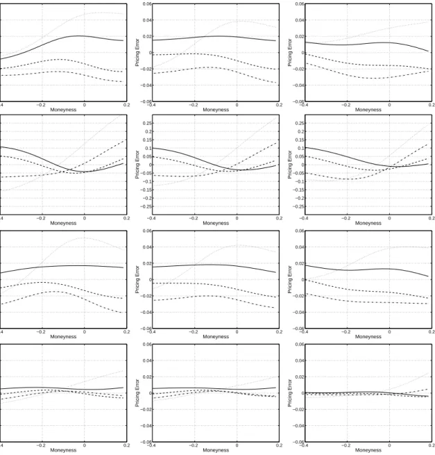
Since the moneyness and maturity of the options vary every day, we estimate the mean option value and the option price variance as percentages of the index level at fixed moneyness and maturities through a nonparametric smoothing method. Refer to Appendix A for details. The left panel of Figure 2 portrays the smoothed mean surface of out-of-the-money option prices. As expected, option prices are the highest for at the money options and they also increase with maturities. The right panel portrays the variance estimates of the option prices. Overall, the variance increases with the maturity of the option. For the same maturity, out-of-the-money puts (k<0) have a smaller variation than out-the-money calls

(k>0). This might be a reflection of different liquidities: OTM puts are more liquid and more heavily traded than OTM calls for S&P 500 index options. Given the estimated variance of the option prices, the optimal weight at each moneyness and maturity level is defined as its reciprocal.

B. Performance Measures

Different models are compared based on the sample properties of the daily mean squared pricing errors (mset) defined in equation (18), under the estimated model parameters. A small sample average of

the daily mean squared errors for a model would indicate that the model fits the option prices well on average. A small standard deviation for a model would further indicate that the model is capable of capturing different cross-sectional properties of the option prices at different dates. Our analysis is based on both the in-sample mean squared errors of the first 139 days and the out-of-sample mean squared errors of the last 150 days. In addition, we gauge the statistical significance of the performance difference between any two models i and j based on the following t-statistic of the sample differences in daily mean squared errors,

t-statistic= mse

i_−msej

stdev(mse_ti−mse_tj)/

√

T

, (20)

where the overline onmsedenotes the sample average andstdev(·)denotes the standard deviation.

III. Model Performance Analysis

We now analyze the parameter estimates and the sample properties of the mean squared pricing errors for each of the 12 models introduced in Section I. As mentioned earlier, our objective is to investigate which jump type and which stochastic volatility specification deliver the best performance in pricing S&P 500 index options. Our analysis below is focused on answering these two questions.

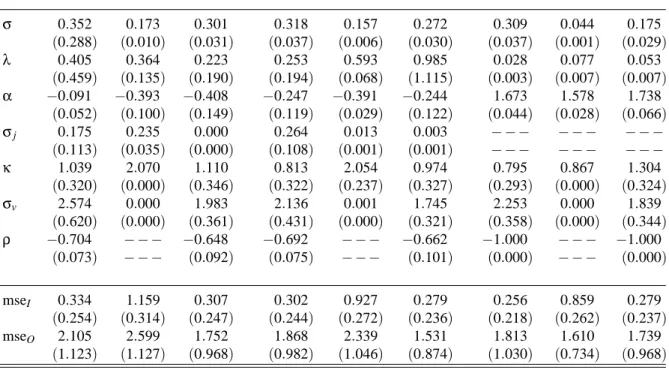
Tables III and IV report the parameter estimates and their standard errors for one-factor (SV1-SV3) and two-factor stochastic volatility (SV4) models, respectively. We also report in the tables the sample average and standard deviation of the daily mean squared pricing errors, both in sample (mseI)

t-statistics for pair-wise model comparisons using (20). The results for the comparison are reported in

Table V. With 12 models, we could have reported a 12×12 matrix of pair-wise t-tests; but to focus on addressing the two questions raised above, we report the t-tests in two panels. Panel A compares the performance of different jump structures under each stochastic volatility specification (SV1 to SV4); Panel B compares the performance of different SV specifications for a given jump structure (MJ, VG, or LS). Both in-sample and out-of-sample comparisons are reported.

A. What Jump Structure Best Captures the Behavior of S&P 500 Index Options?

Since our 12 models are combinations of three jump structures and four SV specifications, we compare the performance of the three jump structures, MJ, VG, and LS, under each SV specification to answer the question on jump types. If the performance ranking of the three jump structures depends crucially on the specific SV specification, the choice of a jump structure in model design should be contingent on the SV specification to be used. On the other hand, if the performance rankings are the same under each of the four SV specifications, we would conclude that the superiority of one jump structure over the others in capturing the behavior of S&P 500 index options is unconditional and robust to perturbations in SV specifications. The empirical evidence favors the latter: the infinite activity jump structures (VG and LS) outperform the classic finite activity compound Poisson (MJ) jump structure under all four SV specifications.

Panel A of Table V addresses the question based on the t-statistics defined in equation (20). Each column in Panel A compares the performance of two jump structures under each SV specification. For example, the column under “MJ−V G” compares the performance of the Merton jump model (MJ)

against the performance of the variance-gamma model (VG), under each of the four SV specifications. In particular, a t-statistics of 1.96 or higher implies that the pricing error from the MJ model is signifi-cantly larger than the pricing error from the VG model under a 95% confidence interval, and hence, the VG model outperforms the MJ model. A t-value of−1.96 or less implies the opposite.

The t-values under column MJ−V G are strongly positive under all SV specifications, both in

sample and out of sample. The same is also observed for all t-tests under the MJ−LS column. Thus, our

jump structure of Merton (1976), performs significantly worse than both the VG and the LS jump structures. This results holds under all of the four SV specifications and for both in-sample and out-of-sample tests. The performance difference between VG and LS, on the other hand, is much smaller and can have different signs depending upon the SV specification assumed. The t-values under the V G−LS

column are much smaller, positive under SV1, SV2, and SV4, but negative under SV3. Carr and Wu (2002a) obtain similar performance rankings for the three jump structures without incorporating any stochastic volatilities. Our results show that this ranking remains unchanged in the presence of stochastic volatility.

The key structural difference between the Merton jump model and the other two types of jump structures lies in the jump frequency specification. Within any finite time interval, the number of jumps under MJ is finite and is captured by the jump intensity measure λ. The estimates for λunder the MJ structure fall between 0.086 under the SV4 specification (see Table IV) and 0.405 under the SV1 specification (see Table III). Specifically, an estimate of 0.405 or smaller implies that on average, one observes one jump every two and half years or so, a rare event. In contrast, under the VG and LS jump structures, the number of jumps under any finite time interval is infinite. One thus expects to observe much more frequent jumps of different magnitudes than in the Merton jump case. Our estimation results indicate that, to capture the behavior of S&P 500 index options, one needs to incorporate a much more frequent jump structure in the underlying return process than the classic Merton model allows.

B. Where Does Stochastic Volatility Come From?

By applying stochastic time changes to different L´evy components, one can generate stochastic volatil-ity from either the diffusion component, or the jump component, or both. It thus becomes a purely empirical issue as to where exactly the stochastic volatility comes from. We address this issue by com-paring the empirical performances of four different stochastic volatility specifications in pricing the S&P 500 index options.

Panel B of Table V compares the performance of the four stochastic volatility specifications under each of the three jump structures. We first look at the three one-factor SV specifications: SV1, SV2, and

SV3. We find that the in-sample t-test values under the “SV 1−SV 2” column are all strongly negative

and that the in-sample t-test values under the “SV 2−SV 3” column are all strongly positive, suggesting

that the SV2 specification is significantly outperformed by the other two one-factor SV specifications. In contrast, the in-sample t-test estimates under the “SV 1−SV 3” column are much smaller and have

different signs under different jump specifications: positive under MJ and VG, negative under LS. The out-of-sample performance comparison delivers similar conclusions, except under the LS jump structure, where the t-statistics are much smaller.

Recall that under the SV2 specification, the instantaneous variance of the diffusion component is constant and all stochastic volatilities are attributed to the time variation in the arrival rate of jumps. Inferior performance of SV2, as compared to SV1 and SV3, indicates that the instantaneous variance of the diffusion component should be stochastic. The parameter estimates of the three one-factor SV specifications in Table III also tell a similar story. The volatility of volatility estimates (σv) are always

strongly positive under SV1 specifications, slightly smaller under SV3 specifications, but are close to zero under SV2 specifications, when only the arrival rate of the jump component is allowed to be stochastic. For example, the estimate ofσv is 2.136 under VGDSV1, 1.745 under VGDSV3, but a

mere 0.001 under VGDSV2. Similar results hold for MJ and LS models. These estimates indicate that, overall, the arrival rate of the jump component is not as volatile as the instantaneous variance of the diffusion component. This evidence supports traditional stochastic volatility specifications but casts doubt on the performance of the stochastic volatility models of Carr, Geman, Madan, and Yor (2001), which generate stochastic volatility from pure jump models.

Another important structural difference between the SV2 specification and the other SV specifica-tions is that SV2 is the only specification where instantaneous correlation is not incorporated between the return innovation and the innovation in the arrival rate. Hence, the SV2 specification cannot cap-ture the widely documented negative correlation between stock returns and return volatilities, i.e., the “leverage effect.”9 Yet, under all other SV specifications, the estimates for this instantaneous correla-tion parameter,ρ, are all strongly negative (see Table III), suggesting the importance of incorporating such a leverage effect in capturing the behavior of S&P 500 index option prices. In particular, this

9_{Black (1976) first documented this phenomenon and attributed it to the “leverage effect;” however, various other}

expla-nations have also been proposed in the literature, e.g., Haugen, Talmor, and Torous (1991), Campbell and Hentschel (1992), Campbell and Kyle (1993), and Bekaert and Wu (2000).

negative correlation helps in generating negative skewness in the conditional index return distribution implied by the option prices.

Consistent with this observation, Carr, Geman, Madan, and Yor (2001) also note that, without the leverage effect, the performance of the SV3 specification declines to approximately the same level as the SV2 specification. Therefore, this lack of negative correlation under SV2 constitutes another key reason for its significantly worse performance compared to other one-factor SV specifications.

In contrast to the three one-factor SV specifications, the SV4 specification allows the instantaneous variance of the diffusion component and the arrival rate of the jump component to vary separately. The

t-statistics in Table V indicate that this extra flexibility significantly improves the model performance.

The t-tests for performance comparisons between SV4 and all the one-factor SV specifications are strongly negative, both in sample and out of sample, indicating that the two-factor SV4 models perform much better than all the one-factor SV models. This superior performance of the SV4 models indicates that stochastic volatility actually comes from two separate sources: the instantaneous variance of the diffusion component and the arrival rate of the jump component.

The superior performance of the SV4 models has important implications in practice. First, it implies that a high volatility day on the market can be due to either intensified arrival of large events or increased arrival of small, diffusive events, or both. The exact source of high volatility is hence subject to further research and shall be case dependent. This result is in contrast to the implication of earlier option pricing models, e.g. Bates (1996) and Bakshi, Cao, and Chen (1997), both of which assume that variations in volatility can only come from variations in the diffusive volatility.

Furthermore, the superior performance of SV4 models also indicate that, of the four SV specifica-tions, SV4 models suffer the least from model misspecification. Hence, comparisons of different jump structures should be the least biased when the comparison is based upon the SV4 framework. The ranking of the three jump structures under SV4 specifications is, from worst to best, MJ<V G<LS,

with the difference between any pair being statistically significant based on the t-statistics. Recall that the jump frequency increases from MJ to VG and to LS. The performance ranking is in line with this ranking of jump frequency for different jump structures. Therefore, we conclude that the market prices

the S&P 500 index options as if the discontinuous index level movements are frequent occurrences and not rare events.

C. How Do the Risk-Neutral Dynamics of the Two Activity Rates Differ?

Since the SV4 specification provides an encompassing framework for all the one-factor SV specifi-cations, we can learn more about the risk-neutral dynamics of the activity rates by investigating the relevant parameter estimates of the SV4 models, which are reported in Table IV.

Based on the square-root specification for the risk-neutral activity rate dynamics, the two elements ofσv= h σd v,σ j v i_>

capture the instantaneous volatility of the two activity rate processes, withσd_v cap-turing the instantaneous volatility of the diffusion variance and σvj the instantaneous volatility of the

jump arrival rate. The estimates indicate that the variance of the diffusion component exhibits larger instantaneous volatility than the arrival rate of the jump component. For example, the estimates forσd_v are 2.417, 2.600, and 4.697 when the jump components are MJ, VG, and LS, respectively. In contrast, the corresponding estimates forσvjare 1.644, 1.433, and 2.582, about half the magnitude forσdv.

On the other hand, the relative persistence of the activity rate dynamics is captured by the two elements of κ=£κd_,κj¤>_{. A smaller value for κimplies a more persistent process. The estimates}

reported in Table IV indicate that the arrival rate of the jump component exhibits a much more per-sistent risk-neutral dynamics than the instantaneous variance of the diffusion component. Specifically, the estimates for κj are 0.002, 0.001, and 0.096, when the jump components are MJ, VG, and LS, respectively, much smaller than the corresponding estimates forκd, which are 2.949, 3.045, and 3.466, respectively.

The parameter estimates for the SV4 specifications indicate that, to match the market price behav-ior of S&P 500 index options, one needs to derive stochastic volatilities from two separate sources: the instantaneous variance of the diffusion component and the arrival rate of the jump component. Furthermore, the risk-neutral dynamics of the diffusion variance needs to exhibit higher instantaneous volatility and much less persistence than the risk-neutral dynamics of the jump arrival rate. Such dif-ferent risk-neutral dynamics for the two activity rate processes dictate that the jump component and the diffusion component play different roles in governing the behavior of S&P 500 options. In particular,