Assessment of MVDR Adaptive Beamforming algorithm in uniform linear arrays, uniform rectangular arrays and uniform circular arrays configurations

ASSESSMENT OF MVDR ADAPTIVE BEAMFORMING ALGORITHM IN

UNIFORM LINEAR ARRAYS, UNIFORM RECTANGULAR ARRAYS AND

UNIFORM CIRCULAR ARRAYS CONFIGURATIONS

Suhail Najm Shahab

1

, Ayib Rosdi Zainun

1

, Nurul Hazilina Noordin

1

and Balasim. S. S.

2 1_{Faculty of Electrical and Electronics Engineering, Universiti Malaysia Pahang, Pekan, Pahang, Malaysia}

2

College of Engineering, University of Anbar, Iraq E-Mail: [email protected]

ABSTRACT

Nowadays, the ever-growing demand for mobile communications is constantly increasing the need for improved capacity, better coverage, and higher-quality service. Whereas three major disabilities limit the capacity and reliability of wireless communication systems; multipath fading, delay spread, and co-channel interference. Beamforming (BF) technique is a powerful means of increasing capacity, data rates and coverage of the wireless cellular communication system. One of the common and widely used approaches to Adaptive Beamforming (ABF) is the Minimum Variance Distortionless Response (MVDR) which can reduce the interference plus noise power without distorting the desired signal. In this paper, MVDR BF with various antenna array geometries includes; uniform linear arrays (ULAs), uniform rectangular arrays (URAs) and uniform circular arrays (UCAs) each consisting of L elements operated in frequency of 2.6 GHz that is implemented in LTE networks were used for analyze and compare the performance of MVDR beamformer. From this study, it is found that the MVDR BF technique with ULA has the best performance and capable of forming adaptive beams with nulling capability towards interfering signals of average null power up to 42.8 dB with improvement on SINR approximately 9% and 11% comparing to UCA. As comparisons, the MVDR technique with ULA is much more accurate than the URA and UCA to null the interference source and steer its radiation lobe with high power towards the desired signal. To evaluate the performance of this work one user with four interferences sources were used through computer simulation by using Matlab.

Keywords: smart antenna, beamforming algorithm, minimum variance distortionless response, linear array, rectangular array, circular array, LTE.

INTRODUCTION

The wireless communications are facing a tremendous challenge to satisfy the ever-increasing demand for capacity. The demand is firstly caused by an increasing number of users but also because of more data intensive applications. By 2016, it is expected to have a numbers of the connected mobile device over 10 billion, exceeding the number of people on Earth, estimated to be 7.3 billion. Personal mobile-ready devices around 8 billion and the remaining 2 billion are machine-to-machine (M2M) connections. The devices will be more powerful and hence can consume and produce more data traffic. From 2011 till 2016, the mobile data traffic will increase 18-fold, tablet traffic 62-fold and streamed content 28-fold. Laptops, smartphones, and other portable devices will handle about 90% of all mobile data traffic by 2016. Remaining 10% belongs to M2M communication and residential broadband mobile gateways, 5% each. Mobile data traffic is expected to outgrow fixed data traffic by three times by the end of 2016 (Calif., 2012).

Interference is one of the main wireless radio communications problems. The interference can be caused by signal itself or by other users (Halim, 2001). The signal can interfere with itself due to multipath components, where the signal is gather with another version of the signal that is delayed because of another propagation path.

Interference from other users can be either unintentional or intentional (Halim, 2001). Unintentional interference is caused by nonidealities in the transmitter or using the same or adjacent channel. Intentional interference or jamming is radiation directed towards a target for the purpose of trying to prevent it from receiving the desired signal. Potential interference in signal processing and telecommunication applications has been a main concern for system designers, and usual filtering techniques are not helpful as the interference signal and desired signal are of the same frequency. Many methods have been adopted to avoid interference, including frequency hopping, but it requires immoderate bandwidth. ABF can solve the problem without the need for additional bandwidth as signals are filtered on the basis of their direction of arrival (DOA). Smart antennas (SAs) possess the capability of suppressing interference signal, so they can improve the signal to interference plus noise ratio (SINR). Array processing utilizes information regarding locations of signal to aid in interference suppression and signal enhancement and is considered the promising technology for interference nulls (Das and Sharma, 2012).

A SA although being a synonym for the adaptive array, it refers to many sets of the antenna, that adaptive array is a part of, which are controlling adaptively. Early publications on the use of smart antenna arrays for

(Howells, 1965). SAs are used nowadays in modern mobile communication systems to enhance the desired and suppress the interference arising due to Co-Channel Interference (CCI), Adjacent Channel Interference (ACI) and multipath. ABF is a ubiquitous task in array signal processing and has been studied widely in the past due to its extensive applications in several areas ranging from radar, sonar, microphone arrays, radio astronomy, seismology, medical diagnosis and treatment, to wireless communications (Allen & Ghavami, 2006; Brandstein and Ward, 2001; Fourikis, 2000; Haykin, Justice, Owsley, Yen, and Kak, 1985; Hudson, 1981; Johnson and Dudgeon, 1993; Li and Stoica, 2005; Van Trees, 2002).

The capacity, data rates, null steering and coverage of the wireless cellular communication system are improved by using various beamforming techniques such as the MVDR. MVDR method is commonly used in ABF, originally proposed by (Capon, 1969) it has been found effective interference and noise reduction while it is needs to know the direction of arrival of impinging signal as the Signal of Interest (SOI) only to maintain the desired signal distortionless while the power of noise and interference minimized in the constraint condition which is basically a unity gain adaptive beamformer.

Adaptive antenna arrays can be forming with varying geometries. In general, they can be classified based on the number of dimensions they extend to; linear (1D), planar (2D), with geometries such as rectangular, circular and hexagonal. The elements can be spaced regularly or irregularly (randomly). Regular spacing is further subdivide into uniform and non-uniform. Typically, the ABF weights are computed to optimize the performance in terms of a certain criterion (Lal Chand Godara, 1997). The earliest studies on improving array performance via geometry optimization date back to the early 1960s. (Unz, 1960) Studied linear arrays and noted that performance improvement could be obtained by holding the weights constant and varying the element positions. In 1960, (King, Packard, & Thomas, 1960) proposed eliminating grating lobes via element placement in an array. In 1961, (Harrington, 1961) considered small element perturbations in an attempt to synthesize a desired array pattern. As the response of the array varies according to DOA, a Steering vector (Sv) is associated with each directional source. The uniqueness of this association depends on array geometry (Lal C Godara and Cantoni, 1981). For a linear array of equispaced elements with element spacing bigger than half of the wavelength, the Sv for every direction is unique (Lal Chand Godara, 2004). Then the beam pattern is formed by adjusting complex weights of the antenna elements so that the beam directed in the direction of interest (Compton, 1988).

So far, little attention has been paid to MVDR ABF with different array topology. In this paper, performance assess of MVDR ABF with uniform linear arrays (ULAs), uniform rectangular arrays (URAs) and uniform circular arrays (UCAs) configurations where the objective is to determine which of the three different

geometries able to offers the best BF capabilities in term of directing the main beam in the direction of the SOI

while placing nulls towards the direction of Signal Not of Interest (SNOI).

The rest of this paper is organized as follows, in section three beamformer design method are described. The simulation outcomes and discussion provided in section four. Finally, section five concludes the paper.

METHODOLOGY

In this part, the mathematical formulation of the design model for adaptive beamforming will be presented in detail. Where consider a single cell with L elements antenna array. Let there are S desired signal sources and I

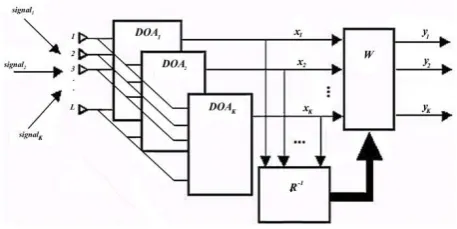
interference sources transmitting on same frequency channel simultaneously. The algorithm starts by constructing a real-life signal model. Consider a number of plane waves from K narrow band sources impinging from different angles (θ, ϕ), the impinging radio frequency signal reaches into antenna array from far field to three different array geometries including; uniform linear arrays (ULAs), uniform rectangular arrays (URAs) and uniform circular arrays (UCAs) with uniform distance between the adjacent elements of d apart. A block diagram of the antenna array using DOA and BF process is depicted in figure 1. As shown in this figure, after the signals received by antenna arrays consisting of the desired signals, the interference signals, and the noise, the first part is to estimate the direction of the arrival of the S signals and I

[image:2.595.313.542.572.686.2]

signals by well-known algorithm developed by capon called MVDR spectrum estimator to determine direction of arrival angles of multiple sources. However, the MVDR estimator algorithm requires knowledge of the number of sources. With the known direction of the source, next it can apply the second part by using MVDR ABF technique that placing a straight beam to S signal and placing nulls in the direction of I signals. Each signal multiplied by adaptable complex weights and then summed to form the system output.

Figure-1. Smart antenna array using beamforming process.

The total signals received by adaptive antenna array at time index, t, become:











I i n i s

T

t

x

t

x

t

x

x

1

)

(

)

(

)

(

(1)











I i n i i s

s

t

a

x

t

a

x

x

1

)

(

)

(

)

(

)

(





(2)

Where xs(t), xi(t),xn(t), denote thedesired signal, interference signal, and noise signal added from White Gaussian noise, respectively. The unwanted signal consists of xi(t)+xn(t) and I is the number of interference sources, the desired angle and interference direction of arrival angles are θs and θi , i=1,2….,I, respectively. a(θs) denote the steering vector or array response for wanted signal while a(θi) refer to the interference signal steering vector or array response for the unwanted signal.

Steering vector is a complex vector



C

LK

containing responses of all elements of the array to a narrowband source of unit power depending on the incident angle; It is given by (Lal Chand Godara, 2004):







































    i s i s i s d L jq d jq jqd i s

e

e

e

a

, , , sin ) 1 ( sin 2 sin ,

1

)

(

  





(3)

where d is the element spacing and q is the wave number, given as:





2



q

(4)

Whereλ is the wavelength of the received signal. The signal xT(t) received by multiple antenna elements is multiply by a series of amplitude and phase (weight vector coefficients) which accordingly adjust the amplitude and phase of the incoming signal. This weighted signal is a linear combination of the data from L elements, resulting in the array output, y(t) at any time t, of a narrowband beamformer is given by:

)

(

)

(

1

t

x

w

t

y

_T L l H







(5)

Where y(t) is the beamformer output, xT(t) is the output of the antenna elements, w is the complex weight vector for the antenna element = [w1, w2, …, wL]

T is

1





L

C

beamforming complex vector. (.)H and (.)T denotes

the conjugate transpose (Hermitian transpose) of a vector or a matrix, the conjugate of complex weights is used to simplify the mathematical notation and transposes operators, respectively.

The covariance matrix, Ry is formed conventionally with unlimited snapshots. However, it is estimated by using limited snapshots signal in the actual application. It can be express as:

L n i H I i i i s H s s

y

a

a

a

a

Id

R

2 1 2 2

)

(

)

(

)

(

)

(























 (6)

)

(

)

(

2 s H s s

s

a

a

R









(7) L n i H I i i i n

i

a

a

Id

R

2 1 2

)

(

)

(

















 (8)

)]

(

)

(

[

x

t

x

t

R

R

R

_y



_s



_in





_{T T}H (9)

Where Ry,

2

s



,



_i2,



_n2, IdL, Rs, Ri+n and E[.] denotes, respectively, the L×L theoretical covariance matrix, power of the desired signal, interference power, noise power, identity matrix, SOI covariance matrix, interference plus noise covariance matrix and expectation operator.

The common formulation of the MVDR beamformer that determine the L×1 optimum weight vector is the solution to the following constrained problem (Souden, Benesty, and Affes, 2010):

]

)

(

[

min



y

t

2

1

)

(

.

.

}

{

)

(

min







H _s

y H

w

P



w

R

w

s

t

w

a



(10)

where P(θ)denote the mean output power, a beam pattern can be given in dB as (Lal Chand Godara, 1997):

)

(

max

)

(

log

20

10

_



P

P

pattren

beam



(11)

)

(

)

(

)

(

1 1 MVDR

s y s H

s y

a

R

a

a

R

w







 



(12)

The output signal power of the array as a function of the DOA estimation, using optimum weight vector from MVDR beamforming method (Haykin, 2002), it gives by MVDR spatial spectrum for angle of arrival estimated by detecting the peaks in this angular spectrum as (Capon, 1969):

)

(

)

(

1

)

(

₁

s y s H MVDR

a

R

a

P









_ (13)

SIMULATION RESULTS AND DISCUSSIONS In this paper, L-element uniform linear array (ULA), uniform rectangular array (URA), and uniform circular array (UCA) configurations added to the beamformer system at the base station (BS). The array receives signals from several spatially separated users. The received signal consists of the useful signal, co-channel interference, and a random noise component. Beamforming technique is employed in the BS to increase the output power of the desired signal and reduce the power of co-channel interference and noise. The ABF performance analysis shows an array of different geometries with even and odd number of elements separated by distance, d=λ/2 at carrier frequency (Fc) of 2.6GHz which is the spectrum band is used since this is the band allocated to LTE operators in Malaysia (Malaysian Communications and Multimedia Commission, 2011). This comparison is aim to find which of the three different geometries, linear, rectangular or circular arrays achieve the best beamforming capabilities to form the main beam in wanted direction and nulls in the directions of interferences. In this section two scenarios are discussed, simulation procedure and system parameters are shown in Table-1.

Table-1. Array geometry and simulation parameters.

Array Type ULAs URAs UCAs

Antenna Isotropic

Fc 2.6 GHz

d, dx, dy λ/2

L

8 (1st sc.)

9 (2nd sc.)

8 (1st sc.) [2 4]&[4

2] 9 (2nd sc.)

[3 3]

8 (1st sc.)

9 (2nd sc.)

SOI 30°

SNOI -60°,-30°, 0° and 60°

Snapshot 300

SNR 10dB

a) The first scenario (1st sc.)

First simulation scenario depicted the results calculated by considered the distance between array elements set to be d=dx=dy=0.5λ as usually used in the most MVDR algorithm where dx anddy are the element spacing in the x-y plane for URA. Figure-2 illustrate four array geometries implemented in this scenario.

Figure-2. ULA, URA and UCA antenna geometries.

ULA, URA and UCA with L eight elements spaced a half wavelength apart is used. The additive noise modeled as a complex zero-mean white Gaussian noise. Four interfering sources are assumed to have DOAs (θi) -60º, -30º, 0º and 60º respectively. The SOI is assumed to be a plane wave from the presumed direction θs = 30º. Figure-3 shows the MVDR DOA spectrum plot for estimated direction of all incoming signals. The obtained results pointed out that received signals identified the SOI

and SNOIs perfectly as assumed. By producing peaks in the directions (θ, 0) of -60º, -30º, 0º, 30º and 60º azimuth angles with zero elevation angles respectively, which is computed using formula (13). Each one of this peaks represents the angle of arrival of the incoming signals.

With the incoming signals direction known or estimated, the next step is to using the MVDR ABF technique to improve the signal performance of the desired target and nullifying interferences directions. Figure-4 and Figure-5 shows the MVDR ABF beampattren for SOI at 30º and SNOIs at -60º, -30º, 0º and 60º respectively. This simulation was repeated for eight elements with an input SNR of 10 dB and array geometries of ULA, URA with (2Row, 4Column), URA with (4Row, 2Column) and UCA. The plots observe that the ULA successfully form nulls at each of the income interference sources, and it provide maximum gain to the look direction of the SOI. On the other hand, UCA also provides nulls to the interference sources whereas the main beam is wide beamwidth and not accurate comparing to ULA. Furthermore, the URA with (2Row, 4Column) achieved better performance than URA with (4Row, 2Column) but only one interference angle is null at 0º and higher sidelobe levels than ULA and UCA.

Figure-4. Line plot – comparison of power response of MVDR with ULA, URA and UCA geometries, L=8,

d=λ/2.

Figure-5. Polar plot - comparison of power response of MVDR with ULA, URA and UCA geometries, L=8,

d=λ/2.

b. The second scenario (2nd sc.)

Second simulation scenario illustrates the results calculated by considered nine elements for ULA, URA, and UCA with the same spacing between elements in the

first scenario. ULA, URA and UCA with the same assumption in the first scenario but URA is consists of (3Row, 3Column). From figure 6 and figure 7, it is found that ULA geometry has the capability to direct the main beam toward look target with narrow beam width compare to UCA and null SNOIs. It is clear that the power directed toward the intended direction using ULA is better than that obtained in UCA by approximately -1.5dB as shown in Figure-6. Nevertheless, the directed zero power (null) toward the unwanted directions using ULA has a small different value comparing to results obtained by UCA.

Moreover, the performance of MVDR with URA topology could not provide nulls to the interference sources while the main beam is very wide beamwidth comparing to ULA and UCA. Additionally, the URA with (2Row, 4Column) give the better performance than URA with (3Row, 3Column) and (4Row, 2Column), this may be due to different sequence of the weights vector between antenna elements. Additionally, comparing the results in Figure-5 and Figure-7, one can see that the MVDR ABF yield the main beam with a more narrow beamwidth. This is, of course, expected due to increasing the number of elements in ULA. Meanwhile, the drawback is rising cost, size, and complexity.

Figure-6. Line plot – comparison of power response of MVDR with ULA, URA and UCA geometries, L=9,

d=λ/2.

Figure-7. Polar plot – comparison of power response of MVDR with ULA, URA and UCA geometries, L=9,

In general, the results obtained by MVDR with ULA geometry is best than these obtained from URA and UCA for all directions as demonstrated in table 2 and table 3 in both scenarios. The output power of ULA in the desired direction is 0 dB (unity gain) in both scenario's and placing nulls in the direction of all undesired interference sources with the average null power of 42.8 dB. In addition, Table 4 shown the directivity of each geometry considered in comparison with MVDR algorithm. As seen from this table, ULA attains the highest directivity since the main beamwidth is the narrowest compare to UCA. Furthermore, the directivity with UCA is higher than in URA. Thus, when the directivity increases its mean a more directional focused antenna. Finally, the output SINR resulted from both scenarios tabulated in Table 5. MVDR with ULA geometry has an improvement on SINR with approximately 9% and 11%, respectively as comparing to UCA in both scenarios due to the ULA has a deeply null to interference sources.

Table-2. Comparison of power output values for SOI at 30° and SNOIs at -60º, -30º, 0º and 60º in first scenario

by using eight elements

DOA Power [dB]

[deg] ULA URA [2

4] URA [4 2] UCA

30° 0.0 -0.1 -0.08 -0.7

-60° -42.6 -12.2 -7.5 -39.0

-30° -46.1 -14.5 -16.9 -41.8

0° -41.9 -33.9 -1.9 -41.3

60° -40.8 -13.8 -2.4 -39.4

Table-3. Comparison of power output values for SOI at 30° and SNOIs at -60º, -30º, 0º and 60º in second

scenario by using nine elements

DOA Power [dB]

[deg] ULA URA [3 3] UCA

30° 0.0 -0.1 -1.5

-60° -44.7 -24.3 -39.1

-30° -43.1 -9.9 -43.0

0° -42.3 -6.3 -42.3

60° -41.5 -6.4 -39.0

Table-4. Directivity comparison between ULA, URA and UCA geometries using MVDR for SOI at 30°.

Array Directivity [dBi] for SOI at 30°

geometries 1st sc. 2nd sc.

ULA 8.6 9.0

URA [2 4] -8.6 -

URA [4 2] -19.3 -

URA [3 3] - -17.3

UCA 7.9 3.6

Table-5. Output SINR for ULA, URA and UCA geometries using MVDR BF for both scenarios.

Array SINR [dB]

geometries 1st sc. 2nd sc.

ULA 36.4 36.7

URA [2 4] 8.5 -

URA [4 2] -1.5 -

URA [3 3] - 2.4

UCA 33.4 32.9

CONCLUSIONS

One of the essential requirements for wireless communication technologies is to be applicable and universally desirable. Initially, antenna array geometry was formed as; linear, rectangular, and circular with different elements equispaced. By comparing the results obtained from MVDR algorithm with different array geometries, revealed that MVDR algorithm has the best-beamformed pattern in suppressing the interferences and noise with narrowest main beamwidth when the array geometry is a ULA comparing to URA and UCA. The UCA produce a beam of a wider beamwidth than the corresponding ULA because the UCA does not have an edge elements with additional major lobe appears in its beampattren in direction θ = 90º. Of the three geometries, ULA outperforms the UCA in term of beamwidth and accuracy of the main beam to the SOI and nulls interference sources with average output SINR value of 36.5dB.

REFERENCES

Allen, B. and Ghavami, M. 2006. Adaptive array systems: fundamentals and applications. West Sussex, England: John Wiley and Sons, Ltd.

Calif., S. J. 2012. Cisco Visual Networking Index Forecast Projects 18-Fold Growth in Global Mobile Internet Data Traffic from 2011 to 2016. from http://newsroom.cisco.com/release/668380/Cisco-Visual- Networking-Index-Forecast-Projects-18-Fold-Growth-in-Global-Mobile-Internet-Data-Traffic-From-2011-to-2016

Capon, J. 1969. High-resolution frequency-wavenumber spectrum analysis. Proceedings of the IEEE, 57(8), 1408-1418.

Compton, R. T. 1988. Adaptive antennas: concepts and performance. Englewood Cliffs, N.J.: Prentice Hall.

Das, S. and Sharma, A. K. 2012. Microwave Drilling of Materials. Bhabha Atomic Research Centre (BARC) News letter, Issue No. (329), 15-21.

Fourikis, N. 2000. Advanced array systems, applications and RF technologies (1st ed.). San Diego: Academic Press.

Godara, L. C. 1997. Application of antenna arrays to mobile communications. II. Beam-forming and direction-of-arrival considerations. Proceedings of the IEEE, 85(8), 1195-1245.

Godara, L. C. 2004. Smart antennas. Boca Raton: CRC press.

Godara, L. C. and Cantoni, A. 1981. Uniqueness and linear independence of steering vectors in array space. The Journal of the Acoustical Society of America, 70(2), 467-475.

Halim, M. A. 2001. Adaptive array measurements in communications (1st ed.). Norwood, M A: Artech House Publichers.

Harrington, R. F. 1961. Sidelobe reduction by nonuniform element spacing. IRE Transactions on Antennas and Propagation, 9(2), 187-192.

Haykin, S. 2002. Adaptive Filter Theory (4th ed.): Prentice Hall.

Haykin, S., Justice, J. H., Owsley, N. L., Yen, J. and Kak, A. C. 1985. Array signal processing (1st ed.). United States: Prentice-Hall, Inc., Englewood Cliffs, NJ.

Howells, P. 1965. Intermediate frequency side-lobe canceller, U.S. Patent No. US3202990 A.

Hudson, J. E. 1981. Adaptive array principles. London: Peter Peregrinus Ltd.

Johnson, D. H. and Dudgeon, D. E. 1993. Array Signal Processing-Concepts and Techniques (1st ed.). Englewood Cliffs: Prentice-Hall.

King, D. D., Packard, R. F. and Thomas, R. K. 1960. Unequally-spaced, broad-band antenna arrays. IRE Transactions on Antennas and Propagation, 8(4), 380-384. Li, J. and Stoica, P. 2005. Robust adaptive beamforming. New York: Wiley Online Library.

Malaysian Communications and Multimedia Commission. 2011. SKMM-MCMC Annual Report. from http://www.skmm.gov.my/skmmgovmy/media/General/pd f/

Souden, M., Benesty, J. and Affes, S. 2010. A study of the LCMV and MVDR noise reduction filters. IEEE Transactions on Signal Processing, 58(9), 4925-4935.

Unz, H. 1960. Linear arrays with arbitrarily distributed elements. IRE Transactions on Antennas and Propagation, 8(2), 222-223.