Journal of Chemical and Pharmaceutical Research, 2014, 6(7):2617-2626
Research Article
CODEN(USA) : JCPRC5
ISSN : 0975-7384
Research and application of estimation method for software cost
estimation based on Putnam model
Ning Jingfeng
1, Jiang Yan
2and Yu Honglei
11
Changchun University of Technology, Changchun, China
2
Changchun Finance College, Changchun, China
_____________________________________________________________________________________________
ABSTRACT
Effective software estimate is the most challenging and the most important activity in a software development project management. Only when using scientific methods to reasonably and reliably estimate the scale, the amount of work and cost of the software project, do the people implement good plan and control. The paper introduces several typical ways of software cost estimate, deeply analyses the model of Putnam, uses the examples to research the scale, the number of labors at the peak and the time of the project to provide information for managers to make positive decisions.
Key words: cost of software; estimation; the model of Putnam
_____________________________________________________________________________________________
INTRODUCTION
Estimation and cost budget are always made together, for cost budget is the purpose of estimate, without estimate, there is no possible to make cost budget. In software industry, software cost estimate is always an arduous task[1].Estimate of software development includes both scale and cost estimate. According to the reasonable estimate result, the paper sets out feasible objective, and weighs the cost, schedule and quality of software, implement effective risk management, and provides powerful basis for managers to make investment decisions[2]. The software project estimate runs through the whole software life development cycle, and also needs continuous improvement, planning, review and follow-up[3、4]. With the information accumulated, compare the actual data with the estimate data, and improve the next estimation[5].
CLASSIFICATION OF SOFTWARE COST ESTIMATION
_____________________________________________________________________________
additive, multiple or exponential, in order to get optimized model algorithm expression form. The typical methodsnot based on the algorithm model are experts estimation, analogy estimation and regression analysis.The combination method of software cost estimation obviously applies various techniques and analysis methods in estimation techniques, which is the trend of software cost estimation, and also the better selection that combines various estimation methods advantages and disadvantages, and adapts to different estimation situations and demands.
Putnam estimation model is the dynamic and multivariable estimation model of workload, which is deduced from manpower distribution of large project. Putnam further studies the original model and improves methods, and explores the potential relations among various factors by collecting data. It uses data identification factor and model to explain the performance of software project, and give enough information for the administrator to make decisions for seeking more profit. Putnam model combines many concepts, such as manpower structure, techniques, environment and process productivity.
ESTABLISHMENT OF PUTNAM MODEL
During the software development project, although the quantity of problems is unknown and limited, it also needs manpower to solve the problems. Take indicatrix K of quantity of problems as total labor cost. The accumulative
labor cost involved in the project
C
(
t
)
, expressed as man year.
C
(
t
)
is null at the beginning of the project, and
monotonously increases towards the total labor cost
K
. The change rate of accumulative labor costdC
dt
, showsthe number of men put into at random time during development. So the accumulative cost at time t is shown as:
ζ
ζ
d
m
t
C
(
)
t(
)
0
∫
=
(1)
Suppose at any given time, the optimized number of men put into the project team is in direct proportion to the number of problems to be solved, and then get the following equation:
)]
(
[
)
(
t
C
K
k
dt
t
dC
−
=
(2)
Among which
k
is proportionality coefficient.Because during the life cycle of the project, one group of engineers are gradually increased their efficiency, the concept of project team study is introduced. The growth trend of solving problems ability is also a favorable factor
for improving work efficiency, which is shown as function
p
(
t
)
. So the change rate of accumulative labor cost can
be supposed to be in direct proportion to
p
(
t
)
. This assumption is described through the following differential equation of first order.
)]
(
)[
(
)
(
t
C
K
t
p
dt
t
dC
−
=
(3)
For this equation from the beginning of the project, i.e.,
t
=
0
to get any given timet
integration, get thefollowing equation:
−
=
K
∫
tp
d
t
C
0
(
)
exp
1
)
(
τ
τ
(4)
Separate variables and make replacement of
u
(
t
)
=
K
−
C
(
t
)
, then get
du
=
−
dC
(
t
)
, when
u
(
0
)
=
K
, then:
∫
−
=
−
td
P
K
C
K
Log
0
)
(
τ
τ
Further assumption on the learning function
p
(t
)
, most of the expression of learning functions are linear, i.e., in direct proportion to time, this linear relationship may be expressed as follow:at
t
P
(
)
=
2
(5)
_____________________________________________________________________________
accumulative labor cost
C
(t
)
becomes:)]
exp(
1
[
)
(
t
K
at
2C
=
−
−
(6)By accumulative cost function By accumulative cost function against time differential, the number of labor of the project can be calculated, namely, manpower function:
)
exp(
2
)
(
t
Kat
at
2m
=
−
(7)This function represents Rayleigh curve, at the beginning of the project (t= 0), its value is 0. Then increase toward the employment peak direction, after the peak, gradually reduced to zero. See Figure 1
Fig. 1: Parameter a’s effect on the labor distribution
From the above Figure we can see: parameter a has the dimension of inverse square of time, which plays an important role in determining of labor peak. The larger a value is, the earlier the occurrence time of peak, and the steeper the labor curve is. Derive manpower function against time, to get its zero value, then the relation between
peak hour d
t
and
a
can be found.a
t
d
2
1
2
=
(8)
ESTIMATION OF LABOR PEAK
During measurement of large software development project, the manpower distribution curve has maximum value, which occurs at the time very near delivery time td, before that time, manpower used in specification description,
design, coding, test and qualified verification; after that, manpower demand is used in maintenance, modification and other site work.
According to equation (8), the labor peak time is related to a. Accordingly, acan be obtained from the peak time as follows:
2
2
1
d
t
a
=
(9)
So the number of men put into the project at peak time is determined by using
2
2
1
d
t
to replace a in Norden/Rayleigh model.
_____________________________________________________________________________
)
2
exp(
)
(
2 2 2
d d
t
t
t
t
K
t
m
=
−
(10)
When d
t
t
=
, labor peak can be obtained, which is also expressed in 0
m
. So the expression on labor peak of project is expressed in:
e
t
K
m
d
=
0
(11)
Among which
K
is the total project cost in the unit of man year,t
d is the delivery time in the unit of year,e
isthe base number of natural logarithm,
m
0 is the number of men employed at the peak.DIFFICULTY ESTIMATION
A difficult project mainly refers to a very urgent task which needs to arrange a number of persons to work concurrently, thus resulting in the development plans difficult to control. Compare with the project not quite difficult, difficult project is more sensitive to disturbance. Generally for the project with relatively longer time limit, the manpower distribution curve is relatively flat. The Norden/Rayleigh function against differential of time gets the following equation:
( )
2
(
1
2
2)
exp(
2)
'
at
at
Ka
t
m
=
−
−
When
t
=
0
( )
2'
2
d
t
K
Ka
t
m
=
=
The rate of
2
d
t
K
is called the degree of difficulty (also known as the coefficient of difficulty), expressed in D:
)
/
:
(
2
year
man
unit
t
K
D
d
=
(12)
This relational expression shows, when there are more labor demands or maybe time arrangement is tight(the value
of
t
d is small), the development of project is more difficult. According to formula (11)d
d
t
e
m
t
K
D
=
2=
0From degree of difficulty D, we can see the difficult project normally demand the relatively higher labor peak number in given development time.
LABOR INCREMENT ESTIMATION
The labor increment is also called labor accelerated speed. It shows the project’s bearable and progressive manpower applied maximum allowable growth rate.
D
relative to the derivative oft
dand K:3
'
2
)
(
d d
t
K
t
D
=
−
(13)
( )
1
2(
2)
'
=
−年
d
t
K
D
(14)
In fact
(
)
'
K
D
is always much smaller thanD
'(
t
d)
.
_____________________________________________________________________________
parameter
3
d
t
K
focuses on a value and remain the value,which might be 8, 15 or 27. This parameter is expressed
in
D
0as:(
2)
3
0
man
/year
t
K
D
d
=
(man/year) (15)The value of
D
0and the developed software property have the following relations:8
0
=
D
new software has many interfaces and is interactive with other software systems.15
0
=
D
new and independent system.27
0
=
D
software re-established from the existing software.Parameter
D
0is called labor increment, which is also called labor accelerated speed.D
0 has great influence onthe shape of the labor distribution curve. The bigger
D
0 is, the steeper the labor distribution curve is, the faster thelabor growth accelerate.
ACCUMULATIVE LABOR COST ESTIMATION
Define accumulative labor cost:
According to formula (6)
(
)
[
1
exp(
)]
2
at
K
t
C
=
−
−
Among which C (with man year as unit) gives the labor cost from the beginning of the project to t time, is the total labor cost of software life cycle (with man year as the unit), while a is Norden coefficient defined by Putnam, it
equals
2
2
1
d
t
(see equation 9), so the accumulative labor cost in the whole cycle is expressed as:)]
2
exp(
1
[
)
(
22
d
t
t
K
t
C
=
−
−
(16)
While the accumulative labor cost in development sub-cycle is expressed as:
( )
)]
2
exp(
1
[
20 2
d d
d
t
t
K
t
C
=
−
−
(17)
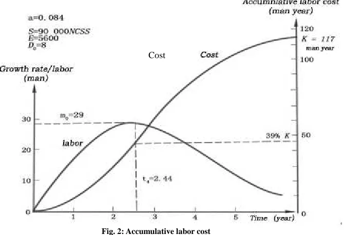
During the period of software project, the accumulative cost increases from zero, then one well known S-curve (see Figure 2) labor costs in delivery time in the management of the project can be obtained in equation (6) by
replacement of
t
=
t
d :( )
K
e
K
t
C
d1
1
=
0
.
39
−
=
(18)
From this equation we can see, the developed software system once delivered to the target processor, on the initial operate stage, it only spends 39% of the total cost K, the rest labor amount uses in acceptance test, maintenance and modification aspects, etc.
DEFINE SOFTWARE EQUATION
The definition of two important parameters of Software projects
K
andt
d, and by means of Rayleigh function,see how labor change with the time, now discuss the relations between
K
andt
d and software products, i.e., tofind the relations between labor cost
K
and development timet
d and the delivered software scaleS
._____________________________________________________________________________
3 2
Pr
=
C
nD
−(19)
[image:6.595.154.489.153.382.2]Pr is productivity, D is the defined degree of difficulty,
C
n is a proportional constant, which depends on the technical condition in the data collecting environment.Fig. 2: Accumulative labor cost
While the degree of productivity is the rate of input to output:
Output
Input
=
Pr
Set productivity Pr is the proportion of the total delivered source codes constituted product and the total labor needed to produce these source codes:
code
of
labor
total
The
code
source
delivered
of
size
The
Pr
=
Total labor includes labor cost spent from the beginning of the project to the delivery time
t
d. From equation (18), we get:( )
t
K
C
d=
0
.
39
(20)Thus, at time
t
d, the delivered software size isS
, use the source program statement number as the unit expressed in:K
S
=
Pr
×
0
.
39
(21)From equations (19)and(21), we get:
3 2
39
.
0
−=
C
KD
S
nAccording to equation(12),we get:
3 2 2
39
.
0
−
=
d n
t
K
K
C
S
after systemizing, we get:
3 4 3 1
39
.
0
C
nK
t
dS
=
(22)
_____________________________________________________________________________
3 4 3 1
d
t
EK
S
=
(23)
E
becomes environment factor, it determined by the technical condition in the production environment. The more efficient of the method and tool of software development, the more skillful the analysts and programmers and their administrators, the higher the environment factoryE
is.K
is the labor cost in the complete period (with manyear as the unit),
t
d is development time (with year as the unit),S
is the scale of the software (with NCSS as the unit).APPLICATION CASE
Take second-hand car trading system as the example. Driven by the state second-hand car policies and logistic promotion policies, the second-hand car markets also have increased gradually, in order to grasp and control the state second-hand car price trend and the region differences, the demands for the second-hand car service platform facing the whole country and with complete functions are also increasing. Because the second-hand car market is characterized as one car one price, one place one price, one person one price, and one time one price, how to judge a car’s actual quality truly and correctly is the inherent problem to increase the second-hand car market close rate to be solved, secondly, how to complete car transaction in different places conveniently, fast, and with high quality to increase the second-hand car market close rate is the key problem to be solved. This project is a project of a certain Changchun second-hand car trading company, mainly realizing the functions such as the management of second-hand car, individual user’s management, enterprise user’s management, and website management. For its cost estimation, relatively mature Putnam model estimation method is used. According to the previous project experience, the estimated scale of this project is 9000NCSS, not more than 18000NCSS (Non-comment source statement), so it belongs to small project, which is developed under the condition of environment factor 1200. This
software is an independent data processing typed program, and its labor acceleration
15
0
=
D
. Determine the development sub-cycle:
The software equation given by equation (23) over E and the third power of which get:
4 3
d
Kt
E
S
=
The right side multiplies and divides
3
d
t
and replaces
3
d
t
K
by labor acceleration
D
0, we get the followingequation:
7 0 3
d
t
D
E
S
=
To solve the development time
t
d, it would get:7 1 3
0
1
=
E
S
D
t
dThis
D
0 value corresponds to the shortest development time, for the above given value, it would get the shortestdevelopment time:
year
t
d
6
.
1
(min)
=
,this value also approximately equals to 1 year and 7 months.
Estimate the labor needed in the complete period. From equation (15) to solve K, it would get:
year
man
7
.
62
3
0
=
=
dt
D
K
From the degree of difficulty defined by equation (12), it would estimate:
year
man
t
K
D
d
/
5
.
24
2
=
=
man/year
_____________________________________________________________________________
at the growth rate of two persons monthly.
Human distribution of software development is a sub –cycle of the complete cycle, it is also Rayleigh function, according to equation (10), described again as follows:
)
2
exp(
.
.
)
(
2 0 2 20d d
d d
t
t
t
t
K
t
m
=
−
(24)
In the formula, d
t
0 is labor peak hour (unit: year), is the labor cost (unit: man year) relevant to the sub-cycle of the
product development, the manpower spent on the development activities of the products, starts after the initial design recheck and stops at the system test and is accepted. Thus it covers the subsystem design, module
specifications, design, coding, test, subsystem test, system test and acceptance.
K
d andt
0d have the following specific value relation:6
k
K
d=
(25)6
0 d dt
t
=
(26)Thus it would get
K
d=10.5 man year. 95% of which would spend on the development period oft
d.According to the accumulative labor cost expression of the time t given by equation (17), it is described again as follows:
−
−
=
2 0 22
exp
1
)
(
d d dt
t
K
t
C
(27)Substitute
t
=
t
d into equation, and divided byK
don both sides of the equation, then it would get:
−
−
=
2 0 22
exp
1
)
(
d d d d dt
t
K
t
C
Then based on equation (26), it would get:
)
3
exp(
1
)
(
−
−
=
d d dK
t
C
thus get:%
95
%
100
)
(
=
×
d d dK
t
C
(28)This means within the delivery time
t
d, 95% of the total development/project labor cost has consumed away, 5%of
K
d leaves for the site installation and qualification testing expenses.So
( )
=
9
.
9
d d
t
C
man year. The rest 0.6 many year (7.2 man months)would spend on after-sales services.
According to the above data, the labor characters used in the development peak hour is calculated. The peak labor time is given from equation (26), so we have:
year
t
t
d d65
.
0
6
0
=
=
or 7.8 months.
Substitute
t
=
t
0d into equation (24), it would get:)
2
1
exp(
)
(
0 00
=
=
−
_____________________________________________________________________________
i.e.
t
e
K
m
d d d
0 0
=
So number of men in peak labor time
m
man
d
8
.
9
0
=
. From the obvious actual consideration, we think thenumber of men in the development team would increase to 10 within 7 months after the project begins.
From the above result,we find, if the time period is short, first, the higher the Norden coefficient
α
value is,the steeper the labor distribution curve is; secondly, labor peak value formula
m
K
t
e
d
=
0 gives higher value,
which is conformed with the former point. This means the more difficult the project is, the more demand to concentrate more persons, and the earlier the concentrate time is. The implicit meaning is, a very urgent task would need to arrange more persons to work concurrently, and making the development plan not easy to control. Compare with not very difficult project, difficult project is more sensitive to the interruption, the slightest demands change or
response result in management will cause the decrease of
2
2
1
d
t
=
α
, i.e., for the project with relatively longertime limit, the manpower distribution curve is relatively flat. Naturally, if the manpower demand is higher, this effect is more obvious.
ESTIMATION RESULT AND COMPARATIVE ANALYSIS
Compare the estimation result with the actual result of the case using Putman model as follow, the accumulative labor cost of the development sub-cycle is 9.9 man year, while the actual one is 12 man year; the estimation result of labor time at the peak is 7.8 months, while the actual time starts in the 10th month after the project begins; the estimation result of the labor number of people at the peak is 10, the actual result is 8. The actual value is basically near the estimated value. In the existing software estimation methods, using the aforementioned experts estimation methods and analogy and other methods, can also estimate the software project. But the expert estimation methods mainly depend on the expert to make the individual judgment by predicting the object future development trend and condition; estimation is able to be made according to the specific software project status, with stronger pertinence, it only depends on the estimation experts’ knowledge and experience, with more subjectivity and lack of objectivity, in actual work, for software project of the same type or even the same software project , different experts might evaluate obvious different results. While during the estimation of software by analogy method, it is the scale estimation by the comparison between new project and history project, which is suitable to evaluate some projects of equivalent application fields, environment and complexity with history project, the precision of its estimation results depend on the integrity and correctness of the history project data.
CONCLUSION
Putnam find that the results get from projects of the same type basically obey the normal distribution, then make linear treatment, then get relevant benchmark graph, using these graphs, development capacity of different software enterprises can be compared, which is very useful for the bidding and progress estimation of project. The paper collects relevant data, makes deeper analysis on Putnam model, and estimates the actual project in second-hand car industry. During using the model estimation, the paper reveals the relations among the source program code length of software project, the development time of software and the workload, with very important theoretical meaning, can help the software administrator to implement effective risk management and decision. The software project estimation methods researched in the paper have verified in many software project, and the results show that these methods have higher reliability and better application potential. But Putnam model also has the properties such as a relatively low correctness, not reflecting the software product, project, participants, and software and hardware resources. In the future estimation process of software project using Putnam model, collecting and accumulating different historical data related to cost estimation, combined by the statistics and analysis of the data to get the model parameter suitable to the organization itself. Software cost estimation is based on probability model, thus it is very difficult to produce precision, but if providing good historical data and using systematic technology, better result can be obtained, completely correct estimation of software cost still needs the continuous efforts from the broad science researchers.
Acknowledgments
_____________________________________________________________________________
REFERENCES
[1]T. C. Jones.Estimating Software Costs, New York:McGraw—Hill, 1998.
[2]B. W. Boehm, R. E. Fairley. Software estimation perspectives, IEEE software,v.17, n.6, pp.22-26, 2000
.
[3]B. Londeix Cost Estimation for Software Development.Reading, MA:AddiSon—Wesley, 1987.[4]R. E. Fairle. Recent advances in Software estimation techniques, In:Proc.1992 Int’l Conf.Software Engineering, New York, ACM Press, pp.382-391, 1992.
[5]B. W. Boehm. Software cost estimation with COCOMO .Englewood Cliffs, NJ:Prentice_Hall, 2000.
[6]Boehm BW, Valerdi R. Achievements and challenges in software resource estimation.Technical Report,
No.USC-CSE-2005-513 , 2005. http://sunset.usc.edu/publications/TECHRPTS/2005/usccse2005-513/usccse
2005-513.pdf
[7]Boehm BW. Understanding and controlling software costs. IEEE Trans. on Software Engineering
,
v.14, n.10, pp.1462-1477, 1988.
[8]R.Agarwal, M.Kumar, Yogesh, et al.Estimating software projects.ACM SIGSOT Software Engineering Notes,
v.26, n.14, pp.60-67, 2001
.
[9]B. W. Boehm. Software Engineering Economics, Englewood C1iffs,NJ:Prentice-Hall, 1981
.
[10]Boehm BW, Valerdi R. Achievements and challenges in software resource estimation, Technical Report,
No.USC-CSE-2005-513, 2005.