Output regulation for discrete time nonlinear stochastic optimal control problems with model reality differences

CONTROL AND OPTIMIZATION

Volume5, Number3, September2015 pp.275–288

OUTPUT REGULATION FOR DISCRETE-TIME NONLINEAR STOCHASTIC OPTIMAL CONTROL PROBLEMS WITH MODEL-REALITY DIFFERENCES

Sie Long Kek

Department of Mathematics and Statistics Universiti Tun Hussein Onn Malaysia

86400 Parit Raja, Malaysia

Mohd Ismail Abd Aziz Department of Mathematical Sciences

Universiti Teknologi Malaysia 81310 UTM, Skudai, Malaysia

Abstract. In this paper, we propose an output regulation approach, which is based on principle of model-reality differences, to obtain the optimal output measurement of a discrete-time nonlinear stochastic optimal control problem. In our approach, a model-based optimal control problem with adding the ad-justable parameters is considered. We aim to regulate the optimal output trajectory of the model used as closely as possible to the output measurement of the original optimal control problem. In doing so, an expanded optimal control problem is introduced, where system optimization and parameter es-timation are integrated. During the computation procedure, the differences between the real plant and the model used are measured repeatedly. In such a way, the optimal solution of the model is updated. At the end of iteration, the converged solution approaches closely to the true optimal solution of the original optimal control problem in spite of model-reality differences. It is im-portant to notice that the resulting algorithm could give the output residual that is superior to those obtained from Kalman filtering theory. The accuracy of the output regulation is therefore highly recommended. For illustration, a continuous stirred-tank reactor problem is studied. The results obtained show the efficiency of the approach proposed.

1. Introduction. Recently, an integrated optimal control algorithm for solving discrete-time nonlinear stochastic optimal control problems has been proposed, see for examples [3], [9], [10] and [4]. The developed algorithm is an iterative approach, where the model-based optimal control problem is solved repeatedly in order to approximate the true optimal solution of the original optimal control problem. With the adjustable parameters that are introduced in the model, the differences between the real plant and the model used could be measured. The repetitive solution is then converged to the real optimal solution within a given tolerance in spite of model-reality differences [11], [12], [1]. On the other hand, because of the present of

2010Mathematics Subject Classification. Primary: 93E20, 93E10; Secondary: 93C10. Key words and phrases. Output regulation, stochastic optimal control, model-reality differ-ences, iterative algorithm, adjustable parameters.

The reviewing process of the paper was handled by Bingsheng He as Guest Editor.

the random disturbances, an optimal filtering solution of the nonlinear stochastic optimal control problem in discrete-time is obtained, where the modified linear quadratic Gaussian optimal control problem is solved repeatedly [5]. In addition to this, a least-square output residual is introduced in the cost functional such that the output error is further minimized [6].

However, minimizing the output error would not give a minimum value of the cost function due to the weighted parameter that is selected for the least-square output residual in the model. In this paper, we propose an efficient computation approach to improve this limitation. In our approach, the linear quadratic regulator optimal control model is considered, where the trajectories of state and control are smoothed in expectation manner. Moreover, an adjustable parameter is introduced to the model output, which is measured from the expected state trajectory. The aim of this adjustable parameter is to regulate the expected output as closely as possible to the real output, as such giving the smallest minimum output error. Note that the Kalman filtering theory is not applied here. It is remarked that the proposed approach gives both of the optimal expected solution and the optimal regulated output at the end of iteration computation procedure despite model-reality differences. Hence, the accuracy of output solution is highly recommended. The rest of the paper is organized as follows. In Section 2, a general class of discrete-time nonlinear stochastic optimal control problem is described. In Section 3, the model-based optimal control problem with the adjustable parameters is dis-cussed. The expectation optimal solution is obtained and then the expected output is regulated approximately to the real output in spite of model-reality differences. In Section 4, an illustrative example of continuous stirred-tank reactor problem is presented to show the efficiency of the proposed approach. Finally, some concluding remarks are made.

2. Problem Description. Consider a general class of stochastic optimal control problem given below:

min

u(k)J0(u) =E[ϕ(x(N), N) +

N−1

X

k=0

L(x(k), u(k), k)]

subject to (1)

x(k+ 1) =f(x(k), u(k), k) +Gω(k)

y(k) =h(x(k), k) +η(k)

where u(k)∈ <m_{,k= 0,1, . . . , N−1,x(k)∈ <}n_{, k= 0,1, . . . , N, andy(k)∈ <}p_,

k = 0,1, . . . , N, are, respectively, the control sequence, the state sequence, and

the measured output. The terms ω(k)∈ <q_{, k = 0,1, . . . , N−1, andη(k) ∈ <}p_,

k= 0,1, . . . , N, are the stationary Gaussian white noise sequences with zero mean

and their covariance matrices are given byQωand Rη, respectively, whereQωis a

q×q positive definite matrix andRη is a p×ppositive definite matrix. Gis an

n×q process noise coefficient matrix,f : <n_{× <}m_{× < → <}n _{represents the real}

plant, and h:<n_{× < → <}p _{is the output measurement, whereasϕ:<}n_{× < → <}

is the terminal cost,L:<n_{× <}m_{× < → <is the cost under summation. Here, J0}

is the scalar cost function andE[·] is the expectation operator. It is assumed that

The initial state is

x(0) =x0

wherex0∈ <n _{is a random vector with mean and covariance given, respectively, by}

E[x0] = ¯x0 andE[(x0−¯x0)(x0−x0¯ )>] =M0.

Here, M0 is an n×npositive definite matrix. It is assumed that the initial state,

process noise and measurement noise are statistically independent.

This optimal control problem is regarded as the real optimal control problem, and is referred to as Problem (P). We notice that the exact solution of Problem (P) is, in general, unable to be obtained. Furthermore, applying the nonlinear filtering theory to estimate the state of the real plant is computationally demanding. In view of these, we propose to solve Problem (P) via solving a simplified model-based optimal control problem iteratively. Let this simplified model-based optimal control problem, which is referred to as Problem (M), be given below:

min

u(k)J1(u) =

1

2x¯(N)

>_{S(N)¯x(N) +γ(N)}

+

N−1

X

k=0

[1

2(¯x(k)

>_{Qx¯(k) +u(k)}>_{Ru(k)) +γ(k)]}

subject to (2)

¯

x(k+ 1) =Ax¯(k) +Bu(k) +α1(k), x¯(0) = ¯x0

¯

y(k) =Cx¯(k) +α2(k)

˘

y(k) = ¯y(k) +α3(k)

where ¯x(k) ∈ <n_{, k = 0,1, . . . , N, ¯y(k) ∈ <}p_{, k = 0,1, . . . , N, and ˘y(k) ∈ <}p_,

k= 0,1, . . . , N, are, respectively, the expected state sequence, the expected output

sequence and the regulated output sequence. Ais ann×nstate transition matrix,

Bis ann×mcontol coefficient matrix,Cis ap×noutput coefficient matrix, while

S(N) and Q aren×npositive semi-definite matrices and R is a m×m positive

definite matrix. Here, γ(k)∈ <, k= 0,1, . . . , N, α1(k)∈ <n_{, k= 0,1, . . . , N−1,}

α2(k) ∈ <p_{, k = 0,1, . . . , N, andα3(k) ∈ <}p_{, k = 0,1, . . . , N, are introduced as} adjustable parameters.

Notice that solving Problem (M) iteratively would give the optimal expected

output solution of Problem (P), which is given by ¯y(k), and the optimal regulated

output solution of Problem (P), which is represented by ˘y(k). Since the Kalman

filtering theory is not used here, the state error covariance is larger than the state error covariance as presented in [5]. However, the additional output measurement, which is added into the model, regulates the expected output sequence as closely as possible to the real output trajectory. In this regulation procedure, we aim to approximate the true output trajectory of Problem (P).

given below:

min

u(k)J2(u) =

1 2x¯(N)

>_{S(N)¯x(N) +γ(N)}

+

N−1

X

k=0

[1

2(¯x(k)

>_{Qx¯(k) +u(k)}>_{Ru(k)) +γ(k)}

+1

2r1ku(k)−v(k)k

2₊1

2r2kx¯(k)−z(k)k

2

+1

2r3ky¯(k)−yˆ(k)k

2_]

subject to (3)

¯

x(k+ 1) =Ax¯(k) +Bu(k) +α1(k), x¯(0) = ¯x0

¯

y(k) =Cx¯(k) +α2(k)

˘

y(k) = ¯y(k) +α3(k)

1

2z(N)

>_{S(N)z(N) +γ(N) =ϕ(z(N), N)}

1 2(z(k)

>_{Qz(k) +v(k)}>_{Rv(k)) +γ(k) =L(z(k), v(k), k)}

Az(k) +Bv(k) +α1(k) =f(z(k), v(k), k)

Cz(k) +α2(k) =h(z(k), k)

ˆ

y(k) +α3(k) =y(k)

v(k) =u(k)

z(k) = ¯x(k)

ˆ

y(k) = ¯y(k)

where v(k)∈ <m_{, k= 0,1, . . . , N −1,z(k)∈ <}n_{, k= 0,1, . . . , N, and ˆy(k)∈ <}p_,

k= 0,1, . . . , N, are introduced to separate the sequences of control, expected state and estimated output in the optimization problem from the respective signals in the

parameter estimation problem, and k · k denotes the usual Euclidean norm. The

terms1₂r1ku(k)−v(k)k2_, 1

2r2kx¯(k)−z(k)k 2_and1

2r3ky¯(k)−ˆy(k)k

2_{withr1∈ <,} r2∈ <andr3∈ <are introduced to improve convexity and to facilitate convergence of the resulting iterative algorithm. It is important to note that the algorithm is

designed such that the constraints v(k) =u(k), z(k) = ¯x(k) and ˆy(k) = ¯y(k) are

satisfied upon termination of the iterations, assuming that convergence is achieved.

The state constraintz(k), the output constraint ˆy(k) and the control constraintv(k)

are used for the computation of the parameter estimation and matching schemes,

while the corresponding state estimate constraint ¯x(k), output estimate constraint

¯

y(k) and control constraint u(k) are used in the optimization of the model-based

optimal control problem. On this basis, the system optimization and the parameter estimation are mutually interactive.

Note that Problem (E) is equivalent to the estimation of Problem (P), which is in terms of expectation and regulation.

H2(k) =1 2(¯x(k)

>_{Qx¯(k) +u(k)}>_{Ru(k)) +γ(k)}

+1

2r1ku(k)−v(k)k

2₊1

2r2kx¯(k)−z(k)k

2

+1

2r3ky¯(k)−yˆ(k)k

2

−λ(k)>u(k)−β(k)>x¯(k)−θ1(k)>y¯(k)

+p(k+ 1)>(Ax¯(k) +Bu(k) +α1(k)) (4)

where λ(k) ∈ <m_{, k = 0,1, . . . , N −1, and β(k) ∈ <}n_{, k = 0,1, . . . , N −1, are}

modifiers. Then, the augmented cost function becomes

J₂0(k) = 1 2x¯(N)

>_{S(N)¯x(N) +γ(N) +p(0)}>_{x¯(0)−p(N)}>_x¯(N)

+ξ(N)(ϕ(z(N), N)−1

2x¯(N)

>_{S(N)¯x(N)−γ(N))}

+Γ>(¯x(N)−z(N)) +θ1(N)>(¯y(N)−yˆ(N))

+

N−1

X

k=0

[He(k)−p(k)>x¯(k) +λ(k)>v(k) +β(k)>z(k)

+ξ(k)(L(z(k), v(k), k)−1

2(z(k)

>_{Qz(k) +v(k)}>_{Rv(k))−γ(k))}

+µ(k)>(f(z(k), v(k), k)−Az(k)−Bv(k)−α1(k))

+θ1(k)>yˆ(k) +θ2(k)>(C¯x(k) +α2(k)−y¯(k))

+θ3(k)>(¯y(k) +α3(k)−y˘(k))

+π1(k)>(h(z(k), k)−Cz(k)−α2(k))

+π2(k)>(y(k)−yˆ(k)−α3(k))] (5)

where p(k), γ(k), ξ(k), µ(k),Γ, λ(k), β(k), πi(k), i = 1,2, and θi(k), i = 1,2,3, are

the appropriate multipliers to be determined later.

Applying the calculus of variation [4], [5], [6], [2], [8], the following necessary optimality conditions are obtained:

(a) Stationary condition:

Ru(k) +B>p(k+ 1)−λ(k) +r1(u(k)−v(k)) = 0 (6a)

(b) Co-state equation:

p(k) =Qx¯(k) +A>p(k+ 1)−β(k) +r2(¯x(k)−z(k)) (6b)

(c) State equation:

¯

x(k+ 1) =Ax¯(k) +Bu(k) +α1(k) (6c)

(d) Boundary conditions:

p(N) =S(N)¯x(N) + Γ and ¯x(0) = ¯x0

(e) Output equations:

¯

(f) Adjustable parameter equations:

ϕ(z(N), N) =1

2z(N)

>_{S(N)z(N) +γ(N) (8a)}

L(z(k), v(k), k) =1 2(z(k)

>_{Qz(k) +v(k)}>_{Rv(k)) +γ(k) (8b)}

f(z(k), v(k), k) =Az(k) +Bv(k) +α1(k) (8c) h(z(k), k) =Cz(k) +α2(k) (8d)

y(k) = ˆy(k) +α3(k) (8e)

(g) Multiplier equations:

Γ =∇z(k)ϕ−S(N)z(N) (9a)

λ(k) =−(∇v(k)L−Rv(k))−

_∂f

∂v(k)−B >

ˆ

p(k+ 1) (9b)

β(k) =−(∇z(k)L−Qz(k))−

∂f ∂z(k)−A

> ˆ

p(k+ 1) (9c)

θ1(k) =r3(¯y(k)−yˆ(k)) (9d)

withξ(k) = 1, µ(k) = ˆp(k+ 1), π1(k) =θ2(k) = 0, and π2(k) =θ3(k) = 0.

(h) Separable variables:

z(k) = ¯x(k), v(k) =u(k),pˆ(k) =p(k),yˆ(k) = ¯y(k) (10)

In view of these optimality conditions, the multipliers are computed from (9), the parameter estimation problem is defined by (8), where the adjustable parameters are calculated, and the modified model-based optimal control problem, which satisfies the optimality conditions in (6) and (7), is given below. This modified model-based optimal control problem is referred to as Problem (MM).

min

u(k)J3(u) =

1 2x¯(N)

>_{S(N)¯x(N) + Γ}>_{x¯(N) +γ(N) +θ1(N)}>_y¯(N)

+

N−1

X

k=0

[1

2(¯x(k)

>_{Qx¯(k) +u(k)}>_{Ru(k)) +γ(k)}

+1

2r1ku(k)−v(k)k

2₊1

2r2kx¯(k)−z(k)k

2

+1

2r3ky¯(k)−yˆ(k)k

2

−λ(k)>u(k)−β(k)>x¯(k)−θ1(k)>y¯(k)]

subject to (11)

¯

x(k+ 1) =Ax¯(k) +Bu(k) +α1(k), x¯(0) = ¯x0

¯

y(k) =Cx¯(k) +α2(k)

˘

y(k) = ¯y(k) +α3(k)

with the specifiedα1(k), α2(k), α3(k), γ(k),Γ, λ(k), β(k), θ1(k), v(k) andz(k), where

the boundary conditions ¯x(0) andp(N) are given with the specified modifier Γ.

Note that it is essential to include the modification termsλ(k)>u(k),β(k)>x¯(k)

andθ1(k)>y¯(k) in the cost function of Problem (MM). Otherwise, the correct

Problem (M) and performing parameter estimation at every iteration step. In addi-tion, to obtain the solution of Problem (MM), it is necessary to solve the two-point boundary-value problem (TPBVP) that is defined by (6b) and (6c).

3.2. Feedback control law. The solution method for solving Problem (MM) is described in Theorem 3.1, where the feedback control law is resulted.

Theorem 3.1. Suppose the optimal control law for Problem (E) exists. Then, this control law is the feedback control law for Problem (MM) given by

u(k) =−K(k)¯x(k) +uf f(k) (12)

where

uf f(k) = (B>S(k+ 1)B+Ra)−1(−B>s(k+ 1)

−B>S(k+ 1)α1(k) +λa(k)) (13a)

K(k) = (B>S(k+ 1)B+Ra)−1B>S(k+ 1)A (13b)

S(k) =Qa+A>S(k+ 1)(A−BK(k)) (13c)

s(k) = (A−BK(k))>(s(k+ 1) +S(k+ 1)α1(k)

−βa(k) +K(k)>λa(k) (13d)

with the boundary conditionsS(N)given ands(N) = 0, and

Ra =R+r1Im, Qa=Q+r2In, λa(k) =λ(k) +r1v(k), βa(k) =β(k) +r2z(k).

Proof. From the necessary optimality condition (6a), we obtain

Rau(k) =−B>p(k+ 1) +λa(k) (14)

Applying sweep method [2], [8],

p(k) =S(k)¯x(k) +s(k) (15)

we substitute (15) fork=k+ 1 into (14), which yields

Rau(k) =−B>S(k+ 1)¯x(k+ 1)−B>s(k+ 1) +λa(k) (16)

Then, substitute the expected state equation (6c) into (16). After some algebraic manipulations, the feedback control law (12) is obtained, where (13a) and (13b) are satisfied.

From the co-state equation (6b), we substitute (15) fork=k+ 1 to give

p(k) =Qax¯(k) +A>S(k+ 1)¯x(k+ 1) +A>s(k+ 1)−βa(k) (17)

Consider the expected state equation (6c) in (17), we obtain

p(k) =Qax¯(k) +A>S(k+ 1)(Ax¯(k) +Bu(k) +α1(k)) +A>s(k+ 1)−βa(k) (18)

Substitute the feedback control law (12) into (18), and doing some algebraic ma-nipulations, it is found that (13c) and (13d) are satisfied after comparing to (15). This completes the proof.

Taking (12) into (6c), the expected state equation becomes

¯

whereas the expected output is measured from

¯

y(k) =Cx¯(k) +α2(k) (20a)

and the regulated output is obtained from

˘

y(k) = ¯y(k) +α3(k) (20b)

3.3. Iterative computation procedure. From the discussion above, the result is summarized as an iterative algorithm, where the computation procedure is given below.

The iterative computation procedure

Data A, B, C, G, Q, R, Qω, Rη, S(N), M0,x0, N, r1, r2, r3, k¯ v, kz, kp, ky, f, L, ϕ, yand

h. Note thatAandB may be chosen based on the linearization of f, andC

is obtained from the linearization ofh.

Step 0 Compute a nominal solution. Assuming thatα1(k) = 0,k= 0,1, . . . , N−1,

α2(k) = 0, k= 0,1, . . . , N,α3(k) = 0, k= 0,1, . . . , N, andr1=r2=r3= 0,

solve Problem (M) that is defined by (2) to obtainu(k)0_{,k= 0,1, . . . , N−1,}

and ¯x(k)0_{, p(k)}0_,y¯(k)0_,y˘(k)0_{, k = 0,1, . . . , N. Then, with α}

1(k) = 0, k =

0,1, . . . , N −1, α2(k) = 0, α3(k) = 0, k = 0,1, . . . , N, and using r1, r2, r3

from the data, computeK(k) andS(k), respectively, from (13b) and (13c).

Seti= 0, v(k)0_=u(k)0_{, z(k)}0_{= ¯x(k)}0_,pˆ(k)0_=p(k)0 _{and ˆy(k)}0_{= ¯y(k)}0_.

Step 1 Compute the parameters γ(k)i_{, k = 0,1, . . . , N, α1(k)}i_{, k= 0,1, . . . , N−1,}

and α2(k)i_{, α3(k)}i_{, k = 0,1, . . . , N, from (8). This is called the parameter} estimation step.

Step 2 Compute the modifiers Γi_{, λ(k)}i_{, β(k)}i_{, k = 0,1, . . . , N−1, andθ1(k)}i_{, k=}

0,1, . . . , N, from (9). Note that this step requires taking the derivatives of

f, handL with respect tov(k)i andz(k)i.

Step 3 Usingα1(k)i, α2(k)i, α3(k)i, γ(k)i,Γi, λ(k)i, β(k)i, θ1(k)i, v(k)i andz(k)i,

s-olve Problem (MM) that is defined by (11) using the result that is presented

in Theorem 3.1. This is called thesystem optimization step.

3.1 Solve (13d) backward to obtains(k)i_{, k= 0,1, . . . , N, and solve (13a), either}

backward or forward, to obtainuf f(k)i, k= 0,1, . . . , N−1.

3.2 Use (12) to obtain the new controlu(k)i, k= 0,1, . . . , N−1.

3.3 Use (19) to obtain the new state ¯x(k)i_{, k= 0,1, . . . , N.}

3.4 Use (15) to obtain the new costatep(k)i_{, k= 0,1, . . . , N.}

3.5 Use (20) to obtain the new output ¯y(k)i _{and ˘y(k)}i_{, k= 0,1, . . . , N.}

Step 4 Test the convergence and update the optimal expectation solution and the optimal output regulation of Problem (P). In order to provide a mechanism for regulating convergence, a simple relaxation method is employed:

v(k)i+1=v(k)i+kv(u(k)i−v(k)i) (21a)

z(k)i+1=z(k)i+kz(¯x(k)i−z(k)i) (21b)

ˆ

p(k)i+1= ˆp(k)i+kp(p(k)i−pˆ(k)i) (21c)

ˆ

y(k)i+1= ˆy(k)i+ky(¯y(k)i−yˆ(k)i) (21d)

where kv, kz, kp, ky ∈(0,1] are scalar gains. Ifv(k)i+1 =v(k)i, k= 0,1, . . .,

N−1,z(k)i+1_=z(k)i_{,k= 0,1, . . . , N, and ˆy(k)}i+1_{= ˆy(k)}i_{,k= 0,1, . . . , N,}

within a given tolerance, stop; else set i = i+ 1, and repeat the procedure

Remarks:

(a) The off-line computation is done, as stated in Step 0, to computeK(k), k=

0,1, . . . , N−1, andS(k), k = 0,1, . . . , N, for the control law design. Then, these parameters are used for solving Problem (M) in Step 0 and for solving Problem (MM) in Step 3, respectively.

(b) The parameters α1(k)i_{, α2(k)}i_{, α3(k)}i_{, γ(k)}i_,Γi_{, λ(k)}i_{, β(k)}i_{, θ1(k)}i _{and s(k)}i

are zero in Step 0. Their calculated values, where α1(k)i_{, α2(k)}i_{, α3(k)}i _and

γ(k)i _{in Step 1, Γ}i_{, λ(k)}i_{, β(k)}i _{and θ1(k)}i _{in Step 2, and s(k)}i _{in Step 3,}

change from iteration to iteration.

(c) The driving input uf f(k) in (13a) corrects the differences between the real

plant and the model used, and it also derives the controller given in (12).

(d) Problem (P) is not necessary to be linear or to have a quadratic cost function.

(e) The conditions v(k)i+1 = v(k)i, z(k)i+1 = z(k)i, and ˆy(k)i+1 = ˆy(k)i are

required to be satisfied for the converged optimal control sequence, the con-verged state estimate sequence and the concon-verged output estimate sequence, respectively. The following averaged 2-norms are computed, and then they

are compared with a given tolerance to verify the convergence of v(k), z(k)

and ˆy(k):

kvi+1−vik2=

1

N−1

N−1

X

k=0

kv(k)i+1−v(k)ik !1/2

(22a)

kzi+1−zik2=

1

N N X

k=0

kz(k)i+1−z(k)ik !1/2

(22b)

kyˆi+1−yˆik2=

1

N N X

k=0

kyˆ(k)i+1−yˆ(k)ik !1/2

(22c)

(f) The relaxation scalars (kv, kz, kp, ky) are step-size that regulates the

conver-gence mechanism. They are normally chosen from the interval (0,1], but this

choice may not result in an optimal number of iterations. It is important

to note that the optimal choice ofkv, kz, kp, ky∈(0,1] is problem dependent,

requiring that the proposed algorithm is run several times from Step 1 to Step

4. These values are initially set askv =kz =kp =ky = 1 for the first run

of the algorithm from Step 1 to Step 4, and then the algorithm is run with different values ranging from 0.1 to 0.9. The value that provides the optimal

number of iterations can then be determined. The parametersr1, r2 and r3

are to enhance convexity, leading to the improvement of the convergence of the algorithm.

4. Illustrative Example. Consider a continuous stirred-tank reactor problem [7]. The real plant is given by

x1(k+ 1) =x1(k)−0.02(x1(k) + 0.25) + 0.01(x2(k) + 0.5) exp

_25x1(k)

x1(k) + 2

−0.01(x1(k) + 0.25)u(k) +ω1(k)

x2(k+ 1) = 0.99x2(k)−0.005−0.01(x2(k) + 0.5) exp

_25x

1(k)

x1(k) + 2

+ω2(k)

x1(0) = 0.05, x2(0) = 0,

and the output measurement isy(k) =x1(k) +η(k), where the expected cost

func-tion

min

u(k)J0(u) = 0.01

N−1

X

k=0

E[(x1(k))2+ (x2(k))2+ 0.1(u(k))2]

is to be minimized. Here,ω(k) = [ω1(k) ω2(k)]>andη(k) are Gaussian white noise

sequences with their respective covariance given byQω= 10−3I2 andRη = 10−3.

This problem is referred to as Problem (P).

To obtain an optimal output solution, which is close enough to the real output, we simplify Problem (P) and propose the following model-based optimal control problem as Problem (M) given below:

min

u(k)

J1(u) =

1 2

N−1

X

k=0

[(¯x1(k))2+ (¯x2(k))2+ 0.1(u(k))2+ 2γ(k)]

subject to

¯

x1(k+ 1) ¯

x2(k+ 1)

=

1.0895 0.0184

−0.1095 0.9716 ¯

x1(k) ¯

x2(k)

+

−0.003

0.000

u(k) +

α11(k)

α12(k)

¯

y(k) = ¯x1(k) +α2(k)

˘

y(k) = ¯y(k) +α3(k)

with the initial condition ¯x(0) = [0.05 0]>, and the adjusted parametersγ(k), α3(k),

α2(k), andα1(k) = [α11(k) α12(k)]>.

After running the iterative algorithm, the simulation result is shown in Table 1, where the iteration number is 19 with the final cost 0.0164. It is almost 99% of the reduction to obtain the optimal cost.

Table 1. Algorithm performance

Iteration Elapsed time Initial cost Final cost

number (s) J∗

1 J19∗

19 2.233 2.0847 0.0164

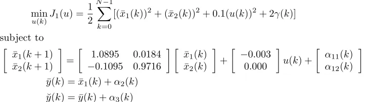
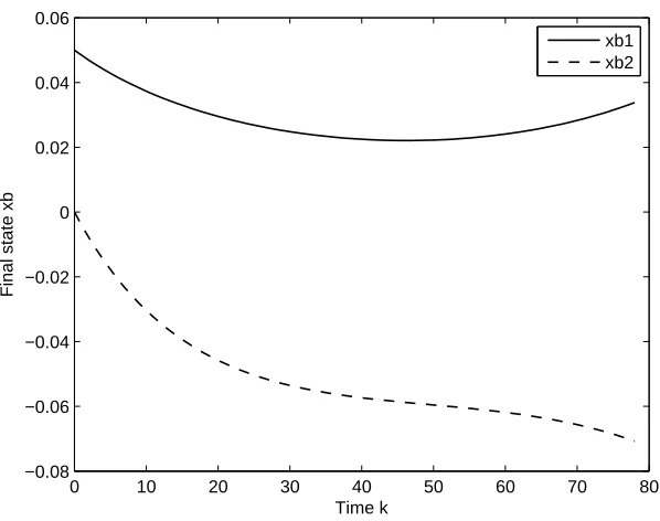
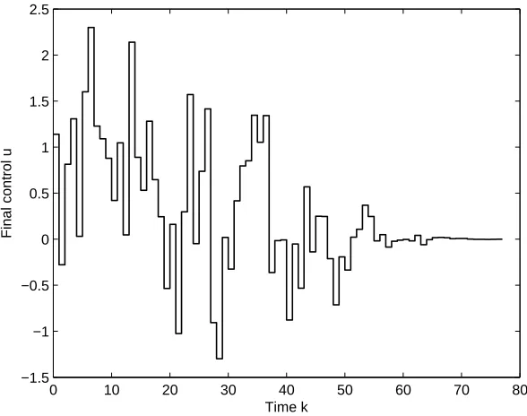
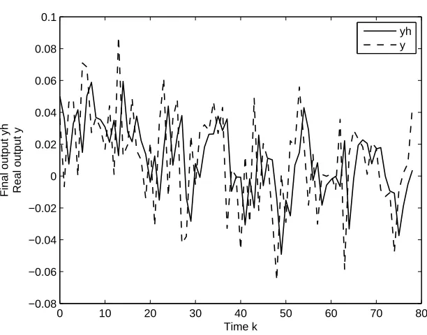
The output residual of the proposed approach is 0.016748, which is smaller than the output residual of the filtering solution given by 0.034731; see [5]. Figures 1, 2 and 3 show, respectively, the trajectories of final control, final state, and final output. From these figures, the trajectories of control and state are smoothly free from disturbance, and the trajectory of output is regulated closely to the real output. These trajectories are then compared to the filtering trajectories of final control, final state and final output as shown in Figures 4, 5 and 6, respectively. It is concluded that the regulated output trajectory tracks the real ouput trajectory efficiently as well as giving the smallest output residual.

0 10 20 30 40 50 60 70 80 0

0.2 0.4 0.6 0.8 1 1.2 1.4 1.6

Time k

Final control u

Figure 1. Final controlu(k) – regulation case

0 10 20 30 40 50 60 70 80 −0.08

−0.06 −0.04 −0.02 0 0.02 0.04 0.06

Time k

Final state xb

xb1 xb2

0 10 20 30 40 50 60 70 80 −0.08

−0.06 −0.04 −0.02 0 0.02 0.04 0.06 0.08 0.1

Time k

Final output yb Real output y

yb y

Figure 3. Final output ¯y(k) and real outputy(k) – regulation case

0 10 20 30 40 50 60 70 80 −1.5

−1 −0.5 0 0.5 1 1.5 2 2.5

Time k

Final control u

0 10 20 30 40 50 60 70 80 −0.06

−0.04 −0.02 0 0.02 0.04 0.06

Time k

Final state xh

xh1 xh2

Figure 5. Final state ¯x(k) – filtering case

0 10 20 30 40 50 60 70 80 −0.08

−0.06 −0.04 −0.02 0 0.02 0.04 0.06 0.08 0.1

Final output yh Real output y

Time k

yh y

regulated output approximates closely to the real output with the smallest output error compared to the filtering solution. It is highly recommended, without applying the Kalman filtering theory, the output regulation solution is prior to the filtering solution and the efficiency of the proposed approach is shown.

REFERENCES

[1] V. M. Becerra and P. D. Roberts,Dynamic integrated system optimization and parameter estimation for discrete time optimal control of nonlinear systems,Int. J. Control,63(1996), 257–281.

[2] A. E. Bryson and Y. C. Ho,Applied Optimal Control, Hemisphere Publishing Company, New York, 1975.

[3] S. L. Kek and A. A. Mohd Ismail, Optimal control of discrete-time linear stochastic dynamic system with model-reality differences inProceeding of International Conference on Machine Learning and Computing (ICML 2009), 10-12 July, 2009, Perth, Australia, 573–578.

[4] S. L. Kek, K. L. Teo and A. A. Mohd Ismail, An integrated optimal control algorithm for discrete-time nonlinear stochastic system,International Journal of Control,83(2010), 2536– 2545.

[5] S. L. Kek, K. L. Teo and A. A. Mohd Ismail,Filtering solution of nonlinear stochastic optimal control problem in discrete-time with model-reality differences,Numerical Algebra, Control and Optimization,2(2012), 207–222.

[6] S. L. Kek, A. A. Mohd Ismail, K. L. Teo and A. Rohanin, An iterative algorithm based on model-reality differences for discrete-time nonlinear stochastic optimal control problems, Numerical Algebra, Control and Optimization,3(2013), 109–125.

[7] D. E. Kirk, Optimal Control Theory: An Introduction, Mineola, NY: Dover Publications, 2004.

[8] F. L. Lewis and V. L. Syrmos,Optimal Control, 2nd ed, John Wiley & Sons 1995.

[9] A. A. Mohd Ismail and S. L. Kek, Optimal control of nonlinear discrete-time stochastic system with model-reality differences, in 2009 IEEE International Conference on Control and Automation, 9-11 December, 2009, Christchurch, New Zealand, 722–726.

[10] A. A. Mohd Ismail, A. Rohanin, S. L. Kek and K. L. Teo, Computational integrated optimal control and estimation with model information for discrete-time nonlinear stochastic dynamic system inProceeding of the 2010 IRAST Internation Congress on Computer Applications and Computational Science (CACS 2010), 4-6 December, 2010, Singapore, 899–902.

[11] P. D. Roberts and T. W. C. Williams,On an algorithm for combined system optimization and parameter estimation,Automatica,17(1981), 199–209.

[12] P. D. Roberts, Optimal control of nonlinear systems with model-reality differences, Proceed-ings of the 31st IEEE Conference on Decision and Control,1(1992), 257–258.

Received May 2014; 1st_{revision January 2015; final revision March 2015.}

E-mail address:[email protected]