MODELING AND CONTROL OF HEAT EXCHANGER BY USING
BIO-INSPIRED ALGORITHM
NUR ATIQAH BINTI DAUD
A project report in partial
fulfillment of the requirements for the award of the
Master‟s Degree of Mechanical Engineering
Faculty Mechanical and Manufacturing Engineering
University Tun Hussein Onn Malaysia
iv ABSTRACT
Heat exchanger is a heat transfer device that is used for transfer of thermal energy
between two or more fluids available at different temperature. Based on the
previous study referred, the same data of heat exchanger had been used but
different types of model were used to find the structural model of heat exchanger.
The main objective of this study is to obtain structural model using ARMAX
equation and optimize the value of PID parameters. In this study, data from heat
exchanger experiment was used to determine the parameter of ARMAX equation
and by using GA and PSO, all the parameters were optimized. Transfer function
obtained will be used for plant modelling. Validation test used to validate between
normalised data input and error. Validation test used were autocorrelation and
cross-correlation. Finally, applying PID controller onto plant modelling to
optimize the value of Kp, Ki and Kd. The analysis shows that MSE value produce from GA is 0.0035473 while PSO‟s MSE value is 0.0043595. ARMAX
parameters were obtained by using GA and PSO with 4 inputs (a0, a1, a2, and a3)
and 4 outputs (b0, b1, b2 and b3). For GA, the inputs are 0.000214, 0.000728,
-0.0020, and -0.000804 while the outputs are -1.0000, -0.1783, -0.1473 and 0.3248.
For PSO, the inputs are 0.0104, -0.0122, -0.0067 and 0.0118 while the outputs are
-0.4274, -0.1256, -0.1865 and -0.2614. From the validation test, GA produced
smoother and effective result compared to PSO with less noise exists. By attaching
PID controller, all the parameters value (Kp, Ki, and Kd) was optimized. For GA,
the parameters are 0.5567, 54.1127 and 0.0005. For PSO, the parameters are
-0.2846, -56.4346 and 0.0010. Even though both algorithms produced different
simulation results, both of them succeed to reduce the result before attaching PID
v ABSTRAK
Penukar haba adalah alat pemindahan haba yang digunakan untuk pemindahan
tenaga haba antara dua atau lebih cecair pada suhu yang berbeza. Berdasarkan
rujukan kajian sebelum ini, data penukar haba yang sama telah digunakan tetapi
berbeza jenis model yang digunakan untuk mencari model struktur. Objektif utama
kajian ini adalah untuk mendapatkan model struktur dengan menggunakan
persamaan ARMAX dan mengoptimumkan nilai parameter PID. Dalam kajian ini,
data dari penukar haba eksperimen telah digunakan untuk menentukan parameter
persamaan ARMAX dan dengan menggunakan GA dan PSO, semua parameter
telah dioptimumkan. Rangkap pindah yang diterima akan digunakan untuk
pemodelan tumbuhan. Ujian validasi digunakan untuk mengesahkan antara input
data pulih dan kesilapan. Ujian validasi yang digunakan adalah autokorelasi dan
silang korelasi. Akhir sekali, memohon pengawal PID ke pemodelan tumbuhan
untuk mengoptimumkan nilai Kp, Ki dan Kd. Analisis menunjukkan bahawa nilai
MSE hasil dari GA adalah 0.0035473 manakala nilai MSE PSO adalah 0.0043595.
Parameter ARMAX diperolehi dengan menggunakan GA dan PSO adalah 4 input
(a0, a1, a2, dan a3) dan 4 output (b0, b1, b2 dan b3). Untuk GA, data masuk
adalah 0.000214, 0.000728, 0.0020, 0.000804 manakala data keluar adalah
-1.0000, -0.1783, -0.1473, 0.3248. Untuk PSO, data masuk adalah 0.0104, -0.0122,
0.0067, 0.0118 manakala data keluar adalah -0.4274, -0.1256, -0.1865, -0.2614.
Daripada ujian pengesahan, GA menghasilkan hasil licin dan berkesan berbanding
dengan PSO dengan kurang bunyi. Dengan melampirkan pengawal PID, semua
nilai parameter (Kp, Ki, dan Kd) telah dioptimumkan. Untuk GA, parameter
-0.5567, -54.1127 and 0.0005. Untuk PSO, parameter -0.2846, -56.4346 and
0.0010. Walaupun kedua-dua algoritma menghasilkan keputusan simulasi yang
berbeza, mereka berjaya untuk mengurangkan hasil keputusan. Kesimpulannya,
vi TABLE OF CONTENTS
TITLE i
DECLARATION ii
DEDICATION iii
ACKNOWLEDGEMENT iv
ABSTRACT v
ABSTRAK vi
TABLE OF CONTENTS vii
LIST OF TABLES x
LIST OF FIGURES xi
LIST OF APPENDICES xiv
CHAPTER 1 INTRODUCTION 1
1.1 Introduction 1
1.2 Problem Statement 2
1.3 Objective 3
1.4 Scope of Study 3
1.5 Expected Outcome 4
vii
CHAPTER 2 LITERATURE REVIEW 6
2.1 Introduction 6
2.2 Heat Exchanger Description 7
2.3 MATLAB Software 10
2.4 System Identification – ARMAX Model 11
2.5 Genetic Algorithm (GA) 16
2.6 Particle Swarm Optimization (PSO) 18
2.7 Correlation 22
2.7.1 Cross-correlation 22
2.7.2 Autocorrelation 23
2.8 PID Controller 24
2.9 Previous Study 26
2.9.1 An ARMAX model of Heat Exchanger
Identification 27
2.9.2 Multiple ARMAX Modelling for Forecasting
Air Conditioning System Performance 27
2.9.3 Dynamic Models for Controllers Design 28
2.9.4 Identification of ARMAX Based On Genetic
Algorithm 29
2.9.5 Identification of the Main Thermal
Characteristics of Building Component Using
MATLAB 30
2.10 Summary of Previous Study 30
CHAPTER 3 METHODOLOGY 31
3.1 Introduction 31
3.2 Heat Exchanger QAD Model BDT921 33
3.3 Plant Description 35
3.4 Experimental Design 41
viii
3.6 Parameter Identification 46
3.7 Optimization of Genetic Algorithm 47
3.8 Optimization of Particle Swarm Optimization 48
3.9 PID Controller 50
3.10 Modeling of Heat Exchanger using GA 50
3.11 Modeling of Heat Exchanger using PSO 52
3.12 Plant of Heat Exchanger 54
3.13 Tuning of PID Controller 55
CHAPTER 4 RESULT AND DISCUSSION 60
4.1 Overview 60
4.2 Genetic Algorithm vs Particle Swarm Optimization 61
4.3 Modelling of Heat Exchanger Plant 64
4.4 Validation Test 69
4.4.1 Validation Test for GA 70
4.4.2 Validation Test for PSO 73
4.5 PID Controller 76
CHAPTER 5 CONCLUSION 80
5.1 Conclusion 80
5.2 Recommendations 81
ix LIST OF TABLES
Tables No. Page
2.1 Properties of Cross-correlation function 23
2.2 Properties of Autocorrelation function 24
3.1 Plant Description of Heat Exchanger QAD model
BDT921 37
3.2 Parameter setting open loop from closed loop system 41
4.1 Summary of GA Analysis Properties 63
4.2 Summary of PSO Analysis Properties 63
4.3 Value of ARMAX Parameters for GA 65
4.4 Value of ARMAX Parameters for PSO 66
4.5 PID Parameters for GA 77
4.6 Step Input Signal Parameters for GA 77
4.7 PID Parameters for PSO 79
x LIST OF FIGURES
Figures No. Page
2.1 Types of heat exchanger 8
2.2 Shell-and-tube exchanger 9
2.3 MATLAB R2010b Version 11
2.4 General Linear Parametric Model 12
2.5 The ARMAX Model Structure 13
2.6 Flowchart of Genetic Algorithm 18
2.7 Flowchart of Particle Swarm Optimization Algorithm 21
2.8 PID Controller in a closed-loop system 25
3.1 Flowchart of the Project 32
3.2 Heat Exchanger QAD Model BDT921 34
3.3 Front view of control panel of the model 35
3.4 Overview of the component in the Heat Exchanger 35
3.5 The schematic diagram of the Heat Exchanger QAD model
BDT921 36
3.6 Tank T13 filled with cold water 37
3.7 Tank T11 of the boiler drum and the heater 38
3.8 Tank T12 filled with preheat water 38
3.9 Temperature Gauge, TG11 38
3.10 Temperature Gauge, TG12 38
3.11 Pump P11 39
3.12 Power Supply (415V/3P) 39
3.13 Pump P14 39
3.14 Temperature Indicating Transmitter, TIT14 39
3.15 Temperature Valve Controller, TCV11 40
xi 3.17 PID Temperature Indicating Controller, TIC11 40
3.18 PID Level/PID Flow Indicating Controller, LIC/FIC11 40
3.19 Block diagram open loop system of heat exchanger QAD
BDT921 41
3.20 Flowchart of the operation process 43
3.21 Recorder data from Recorder LFTR11 45
3.22 Flowchart of Parameter Identification 46
3.23 The optimization flowchart of GA technique 47
3.24 Flowchart of plant modeling using GA 51
3.25 Flowchart of plant modeling using PSO 53
3.26 Plant Modeling for GA and PSO 54
3.27 Plant Modeling with PID controller for GA and PSO 55
3.28 PID Tuner window in MATLAB without parameters 56
3.29 PID Tuner window in MATLAB with parameters 56
3.30 Flowchart of the PID tuner process 57
4.1 MSE value for GA 62
4.2 MSE value for PSO 63
4.3 Sinewave Standard Signal 67
4.4 Comparing graph of „yhat‟ and ‟woo‟ for GA 68
4.5 Comparing graph of „yhat‟ and ‟woo‟ for PSO 68
4.6 GA‟s autocorrelation test 70
4.7 Cross-correlation of input and residual for GA 70
4.8 Cross-correlation of input square and residual for GA 71
4.9 Cross-correlation of input square and residual square for
GA 71
4.10 Cross-correlation of residual and (input*residual) for GA 72
4.11 PSO‟s autocorrelation test 73
4.12 Cross-correlation of input and residual for PSO 73
4.13 Cross-correlation of input square and residual for PSO 74
4.14 Cross-correlation of input square and residual square for
xii 4.15 Cross-correlation of residual and (input*residual) for PSO 75
4.16 Step Standard Signal 76
4.17 The best graph result of PID controller for GA 78
xiii LIST OF APPENDICES
1 CHAPTER 1
INTRODUCTION
1.1 Introduction
Heat exchanger is a heat transfer device that is used for transfer of
thermal energy between two or more fluids available at different temperature. It is
commonly used in industries in almost all process and power plants to generate
steam for the main purpose of electricity to generation via steam turbines
(Yiu,2007). In most heat exchangers, the fluids are separated by a heat transfer
surface, and ideally they do not mix or in direct contact. Common examples of
heat exchangers are familiar to us in day-to-day use are automobile radiators,
condensers, evaporators, air preheaters, and oil coolers (Sha,2003).
The most commonly used types of heat exchanger in industries are
shell and tube heat exchanger. It consists of a bundle of tubes and a shell. One
fluid that needs to be heated or cooled will flows through the tubes and the second
fluid runs over the tubes that provides the heat or absorbs the heat required
(Sha,2003). Heat transfer for both fluids are depends on its flow velocity. The
primary heating medium commonly used for heat exchanger is water vapor
2 process of heat transfer have a boiler to produce water vapor and the cooling
medium that usually used is also water.
During the process, the heating medium will flow through the inlet
tube shell of heat exchanger while the cooling medium will flow through the outer
shell which surrounds the tube of heat exchanger. As mentioned before, both
heating and cooling medium will not mix together. It is mean that there are two
tubes and vessels inside the heat exchanger where the heating medium will flow
using the inside tube while the cooling medium flow using the outside tube of heat
exchanger.
The hot fluid transfers its heat to a conductive surface between it and
cold chamber; subsequently the partition transfers the heat to the cold fluid. This
follows the second law of thermodynamics which states that the heat always flows
from a higher to a lower temperature. The real system of heat exchanger that will
be used in this project is a shell and tube type of heat exchanger. The detail flow
process of heat exchanger will be deeply discussed in Chapter 2.
1.2 Problem Statement
From previous research, in order to identify a model structure of heat
exchanger, a lot of methods had been used such as ARMAX method, RELS
method, AR method and polynomial method to derive the relationship between
input and output obtained. It uses the same data but different types of model.
In this project, method that will be used in order to find the structural
3 Swarm Optimization (PSO) will be used to optimize the values of each parameter
involves. Both structural models will be compared to see its validation using
autocorrelation and cross-correlation. If both structural fit perfectly, the project
will then be continue with applying the PID controller.
1.3 Objective
In order to accomplish this project, there are a few objectives that have to be
achieved. The objectives include;
1. To obtain a mathematical model of heat exchanger by using ARMAX
equation.
2. To validate input and output data value from heat exchanger.
3. To obtained the value of Kp, Ki and Kd of PID controller in order to control
the system.
1.4 Scope of study
The scopes of this study include;
1. Implement ARMAX model in heat exchanger
2. Optimize parameters using Genetic Algorithm (GA) and Particle Swarm
Optimization (PSO).
3. Validate the model with autocorrelation and cross-correlation test.
4 1.5 Expected Outcome
The expected result of this project is to design the experiment and
obtain the data of Heat Exchanger through experimental design. The data obtained
is used to find the transfer function of plant. Another approach that will be used to
find transfer function is using ARMAX model. During the process, Genetic
Algorithm (GA) and Particle Swarm Optimization (PSO) will be used to optimize
the parameters value of ARMAX model. Therefore, we could obtain the parameter
values and hence the transfer function between plant and ARMAX model can be
compared.
1.6 Organisation of Dissertation
The content of this dissertation are organized into three chapters for
this Master Project 1 and each chapter is written to be largely self-contained and
complete.
Chapter 1 will go through the introduction about heat exchanger basic
process. The idea is to be able to understand how the heat exchanger works.
Hence, the process of obtaining data from the machine is much easier.
Furthermore, the problem statement of this project also discussed as a guideline
how the project will carry out to overcome the problem. Next, the research
objectives and the research scopes are defined.
Before performing the detail of project process, detail explanation
about the heat exchanger process will be discussed in Chapter 2. Furthermore,
5 examples, the identification system involved, the optimization system used and the
validation test upon the result produced. The important parts are the previous
works done by other researchers are explored.
For Chapter 3, it describes the methodology involves in conducting
the project in order to achieve the objectives of the project. The detail about plant
description and experiment design will be discussed in this chapter. Furthermore,
summary of genetic algorithm (GA) and particle swarm optimization (PSO)
process also will be include to show the process during optimization of parameter
involves.
For Chapter 4, it described the result obtained and discussed the cause
of it. The detail about analysis of result will also be discussed in this chapter. The
important part is, we can compared the result obtain for GA and PSO.
Furthermore, we can also compare the plant results with and without PID
controller. Parameters of ARMAX model and PID controller also could be
optimized.
For Chapter 5, it described the conclusion and recommendations of
this project. The conclusion is important to conclude all the result obtained. The
6 CHAPTER 2
LITERATURE REVIEW
2.1 Introduction
The needs for energy and materials savings, as well as economic
incentives, have prompted the need to develop more efficient heat exchangers. A
preferred approach to the problem of increasing heat exchanger efficiency, while
maintaining minimum heat exchanger size and operational cost, is to increase heat
exchanger rate.
The heat exchanger is a device built for efficient heat transfer from
one fluid to another, whether the fluids are separated by a solid surface or the
fluids are directly contacted. One of the heat exchanger types that are commonly
used in the process is shell and tube exchanger. For this project, the real system of
heat exchanger that will be used is the shell and tube exchanger type.
These types of heat exchanger are widely used in process industrial
applications. It is the most versatile and used in conventional and nuclear power
stations as condensers, steam generators in pressurized water reactor power plants,
and feed water heaters. They offer great flexibility to meet almost any service
requirement. It can also be designed for high pressures relative to the environment
7 heat exchanger types offer in the industry. The other types of heat exchanger will
be explained in the next subtopic.
2.2 Heat Exchanger Description
A heat exchanger is a device that is used for transfer of thermal energy
(enthalpy) between two or more fluids, between a solid surface and a fluid, or
between solid particulates and a fluid, at differing temperatures and in thermal
contact (Ogata, 1998). The fluids may be single compounds or mixtures. Typical
applications involve heating or cooling of a fluid stream, evaporation or
condensation of a single or multicomponent fluid stream, and heat recovery or heat
rejection from a system (Chong,2000).
A heat exchanger consists of heat exchanging elements such as a core
or a matrix containing the heat transfer surface, and fluid distribution elements
such as headers, manifolds, tanks, inlet and outlet nozzles or pipes, or seals.
Usually there are no moving parts in a heat exchanger; however, there are
exceptions such as a rotary regenerator (in which the matrix is mechanically
driven to rotate at some design speed), a scraped surface heat exchanger, agitated
vessels, and stirred tank reactors (Kakac,2012).
In most heat exchangers, the fluids are separated by a heat exchanger
surface, and ideally they do not mix. Although heat flows from hot fluid to cold
fluid by thermal conduction through the separating wall, heat exchangers are
basically heat convection equipment. Convection within a heat exchanger is
always forced, and may be with or without phase change of one or both fluids. The
basic designs for heat exchangers are the shell-and-tube heat exchanger and the
plate heat exchanger, although many other configurations have been developed.
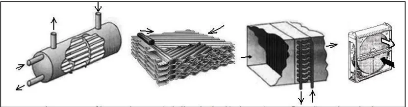
8 a) Shell-and-tube heat exchanger (STHE), where one flow goes along a bunch of
tubes and the other within an outer shell, parallel to the tubes, or in cross flow.
Figure 2.1a shows a typical example of STHE.
b) Plate heat exchanger (PHE), where corrugated plates are held in contact and
the two fluids flow separately along adjacent channels in the configuration.
Figure 2.1b shows details of the interior of a PHE.
c) Open-flow heat exchanger, where one of the flows is not confined within the
equipment. They originate from air-cooled tube-banks, and are mainly used for
final heat release from a liquid to ambient air, as in car radiator, but also used
in vaporizers and condensers in air-conditioning and refrigeration applications,
and in directly fired home water heaters. Figure 2.1c shows the example of
open-flow heat exchanger.
d) Contact heat exchanger, where the two fluids enter into direct contact.
Furthermore, the contact can be continuous such as when the two fluids mix
together and then separate by gravity forces, as in a cooling tower, or the
contact can be alternatively with a third medium, usually solid, as in
regenerative heat exchangers, like the rotating wheel. Figure 2.1d shows the
[image:19.612.143.559.484.594.2]hot gas heats the wheel whereas the cold gas retrieves that energy.
Figure 2.1: Types of heat exchanges: a) shell-and-tube, b) plates, c) open-flow,
d) rotating-wheel (Thulukkanam,2000).
For this project, we are focusing on shell-and-tube exchanger types.
9 mounted in a cylindrical shell with the tube axis parallel to that of the shell. One
fluid flows inside the tubes, the other flows across and along the tubes. The major
components of this exchanger are tubes (or tube bundle), shell, front-end head,
[image:20.612.143.560.195.374.2]rear-end head, baffles, and tube sheets.
Figure 2.2: Shell-and-tube exchanger (Thulukkanam,2000).
Varieties of different internal constructions are used in shell-and-tube
exchangers, depending on the desired heat transfer and pressure drop performance
and the methods employed to reduce thermal stresses, to prevent leakages, to
provide for ease of cleaning, to contain operating pressures and temperatures, to
control corrosion, to accommodate highly asymmetric flows, and so on (Chong
2000). They are the most versatile exchangers made from a variety of metal and
nonmetal materials (graphite, glass, and Teflon) and in sizes from small (0.1m²,
1ft²) to super giant (over 100,000m², ft²) (Thulukkanam,2000). Here are the
main advantages of shell-and-tube heat exchanger:
a) Condensation or boiling heat transfer can be accommodated in either the tubes
or the shell, and the orientation can be horizontal or vertical.
10 c) Thermal stresses can be accommodated inexpensively.
d) The shell and tubes can be made of different materials.
e) Cleaning and repair are relatively straightforward, because the equipment can
be dismantled for this purpose.
Therefore, the shell-and-tube heat exchangers are widely used in the industry since
it offers a great flexibility to meet almost any service requirement.
2.3 MATLAB Software
The high-performance language for technical computing
integrates computation, visualization, and programming in an easy-to-use
environment where problems and solutions are expected in familiar mathematical
notation. It is high-level technical computing language and interactive
environment for algorithm development, data visualization, data analysis, and
numeric computation. MATLAB is stands for matrix laboratory and is used in a
wide range of applications. It is was originally written to provide easy access to
matrix software developed by the LINPACK and EISPACK projects, which
together represent the state-of-the-art in software for matrix computation.
It features a family of application-specific solutions called toolboxes.
Very important to most users of MATLAB, toolboxes allow people to learn and
apply specialized technology. Toolboxes are comprehensive collections of
functions (M-files) that extend the environment to solve particular classes of
problems. Areas in which toolboxes are available include signal processing,
control systems, neural networks, fuzzy logic, wavelets, simulation, and many
11 Figure 2.3: MATLAB R2010b Version
2.4 System Identification – ARMAX Model
System identification is the general process of developing a model for
some particular system from given input-output data and the process of deriving a
mathematical system model from observed data in accordance with some
predetermined criterion. To solve this system identification, there are a lot of
structures such as ARX (Autoregression with exogenous input) model, ARMAX
(Autoregression moving average exogenous input) model, OE (Output Error)
model and general polynomial model. In this project, the selected model structure
that will be used is ARMAX model and estimation algorithm using Genetic
Algorithm (GA) and Particle Swarm Optimization (PSO).
The model for this identification is heat exchanger QAD BDT 921.
For model validation, the identified model will be test using autocorrelation test
and cross-correlation test. It is to verify that the identified model fulfills the
modeling requirement according to subjective and objective criteria of good model
12 designed identification experiment, where the user may determine which signals to
measure them and may also choose the input signals. The objective with
experiment design is thus to make these choices so that the data become
maximally informative, subject to constraints that may be at hand. In other cases
the user may not have the possibility to effect the experiment, but must use data
from the normal operation of the system.
Parametric system identification is the fitting of model parameters to a
pre-selected model by using input output data. The qualitative information by
non-parametric can be used to select the proper model structure. Parametric
identification can be seen as identifying the optimal parameters of a filter of
pre-determined order. The parameter identified by the system is the best
approximation to the real model parameters with respect to a certain criteria such
as the minimum of norm between the estimate and validation. Most of the
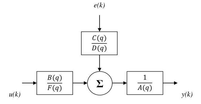
parametric methods can be described as variant of the general linear parametric
[image:23.612.185.521.432.607.2]model for single-output system in Figure 2.4.
Figure 2.4: General Linear Parametric Model
Where the discrete shift operator, u(k) is the input, e(k) is the noise and
disturbance, y(k) is the output and A(q), B(q), C(q), D(q) and F(q) are polynomials e(k)
𝐶(𝑞) 𝐷(𝑞)
𝐴(𝑞) 𝐵(𝑞)
𝐹(𝑞)
u(k) y(k)
13 in shift operator (z or q). The general structure is defined by giving the time-delays
and the orders if the polynomials.
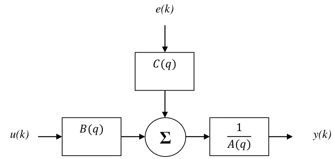
In this project, ARMAX (Autoregressive moving average exogenous)
is selected as a model structure. The structure of an ARMAX model is show below
[image:24.612.183.524.225.388.2]in Figure 2.5.
Figure 2.5: The ARMAX Model Structure
The ARMAX model structure is equation (2.1),
( ) ( ) ( )
( ) ( )
( ) ( ) ( ) (2.1)
Where:
y(t): Output at time t
: Number of poles
: Number of zeroes plus 1
: Number of C coefficients
e(k)
𝐶(𝑞)
𝐴(𝑞) 𝐵(𝑞)
14 : Number of input samples that occur before the input affects the output.
Also called the dead time in the system.
( ) ( ): Previous outputs on which the current output
depends
( ) ( ): Previous and delayed inputs on which the
current output depends
( ) ( ): White-noise disturbance value
The models constitute an important class of difference equation on the form in
equation (2.2) (Kachitvichyanukul 2012).
( ) ( ) ( ) (2.2)
Where d is s time delay and A, B, C are polynomials as equation (2.3).
( )
( )
( )
(2.3)
The parameters na, nb, and nc are the orders of the autoregressive ARMAX
model, and nk is the delay, q is the delay operator. The adjustable parameters are
written in equation (2.4).
(2.4)
Only special case of the ARMAX model that admits a reformulation to the linear
regression model is the controlled autoregressive model (ARX) as the equation
(2.5).
15 Where ek is white noise. Hence, there is no immediate reformulation of the
general ARMAX model that results in a linear regression model
unless the disturbances {ek} are available to measurement.
The ARMAX models include several interesting special cases such as the
autoregressive (AR) model. If the data is a time series, which has no input
channels and one output channel, then armax calculates an ARMAX model for the
time series as an equation (2.6).
( ) (2.6)
This is effective to model harmonics confounded with noise. The moving average
(MA) model that is show in equation (2.7),
( ) (2.7)
is another type that is popular in signal processing as a basic for filter design (FIR)
and the identification of truncated impulse responses. The ARMAX model
equation is show in equation (2.8).
( ) ( ) (2.8)
The mathematical expression of the generalized structure is written in equation
(2.9).
( ) ( ) ( ) ( ) ( ) ( ) ( ) (2.9)
An ARMAX model structure includes disturbance dynamics.
ARMAX models are useful when have dominating disturbances that enter early in
16 coefficients in the ARMAX model structure which is A, B and C polynomials. An
ARMAX has been selected in this project because it has a suitable model structure
that can give an accurate data which can be to compare the output, input and error
data and it is a model that explains a dependent variable out of lagged
(Hannan,1980).
2.5 Genetic Algorithm (GA)
The concept of genetic algorithm (GA) was developed by Holland and
his colleagues in the 1960s and 1970s (Holland,1975). GA is inspired by the
evolutionist theory that explains the origin of species. Basically, in nature the
weak and unfit species within their environment will face with extinction by
natural habits. The strong and capability ones have greater opportunity to pass
their genes to future generations via reproduction. Occasionally, when the
evolutions of gene process are slow, random changes within the population may
occur. If the new species that evolve from the old one have their additional
advantages, they may succeed in the survival challenge. The unsuccessful one will
be eliminated by the natural selection.
Genetic Algorithms are search and optimization techniques inspired by two biological principles namely the process of “natural selection” and the mechanics of “natural genetics” (Hong,2002). GAs will manipulate not only one
potential solution to a problem but a lot of potential solutions which called as
population. The potential solution is refer to chromosomes and chromosomes are
represents all the parameters of the solution. Each chromosomes will be compared
each other in the population and fitness between them indicates the successful
17 GA operates with a collection of chromosomes, called a population.
Typically, it initialized with a random population consisting of between 20 to 100
individuals. As the search evolves, the population includes fitter and fitter
solutions, and eventually it converges, meaning that it is dominated by a single
solution. Holland also presented a proof of convergence (the scheme theorem) to
the global optimum where chromosomes are binary vectors (Holland,1975). There
are three main stages of a genetic algorithm; these are known as reproduction,
crossover and mutation (Ibrahim,2005). All main stages will be explained below:
a) Reproduction: During the reproduction phase, the fitness value of each
chromosome is assessed. This value is used in the selection process to provide
bias towards fitter individuals. Just like in natural evolution, a fit chromosome
has a higher probability of being selected for reproduction.
b) Crossover: Once the selection process is completed, the crossover algorithm is
initiated. The crossover operations swap certain parts of the two selected
strings in a bid to capture the good parts of old chromosomes and create better
new ones. Genetic operators manipulate the characters of a chromosome
directly, using the assumption that certain individual‟s gene codes, on average,
produce fitter individuals.
c) Mutation: Mutation operator introduces random changes into characteristics of
chromosomes. Mutation is generally applied at the gene level. In typical GA
implementations, the mutation rate is very small typically less than 1%.
Therefore, the new chromosome produced by mutation will not be very
different from the original one.
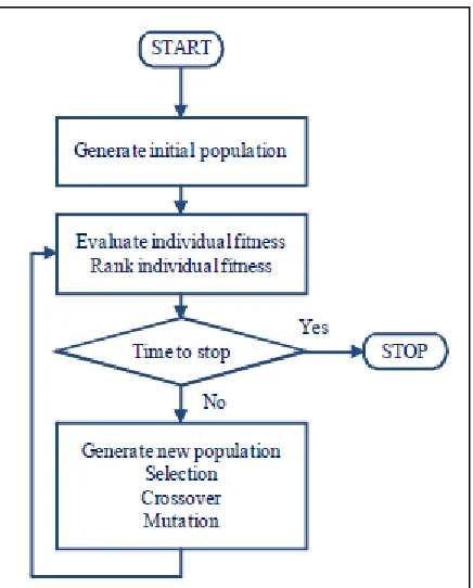
The main idea of GA is to mimic the natural selection and the survival
of the fittest. In GA, the solutions are represented as chromosomes. The
chromosomes are evaluated for fitness values and they are ranked from best to
worst based on fitness value. The process is shown in Figure 2.6 below
18 Figure 2.6: Flowchart of Genetic Algorithm (Kohn,1998).
The process starts with better chromosomes are selected with higher
probabilities than the chromosomes with poorer fitness. The selection probabilities
are usually defined using the relative ranking of the fitness values. Once the parent
chromosomes are selected, the crossover operator combines the chromosome of
the parents to produce new offspring. Since fitter individuals are being selected
more often, there is a tendency that the new solutions may become very similar
after several generations, and the diversity of the population may decline; and this
could lead to population stagnation. Mutation is a mechanism to inject diversity
19 2.6 Particle Swarm Optimization (PSO)
The Particle Swarm Optimization is one of the stochastic optimization
techniques. PSO is based on the social and personal behavior of a swarm. It was
first introduced by Eberhart and Kennedy (Kennedy,2001). The researcher
described how PSO can be applied to a nonlinear optimization problem through
the simulation of a social system characterized by swarms. PSO would
continuously search for a new position for each swarm based on their social best position and self best position. The word “swarm” comes from the irregular
movements of the particles in the problem space, now more similar to a swarm of
mosquitoes rather than a flock of birds or a school of fish (Valle,2006).
PSO and evolutionary computation techniques, like a Genetic
Algorithm, are especially similar. Both algorithms would work by searching
solutions enhanced with updating generations. However, there is nothing to the equivalent of „evolution operators‟ in PSO, which is common in Genetic
Algorithm (Engelbrecht 2006). PSO is also being used in system identification
problems. Huang and colleagues have demonstrated that PSO can be used for
identifying as ARMAX model for Short-term Load Forecasting (Huang,2005).
The basic of PSO algorithm is described by Equation 2.10 and Equation 2.11
(Gautam,2010).
[ ] (2.10)
(2.11)
Where:
: Position of the particle during iteration.
: Velocity of the particle during iteration.
20 w: Inertial coefficient
: Cognitive and social parameters.
: Random numbers between 0 and 1.
Noted that Equation 2.10 is the summation of three different velocities updates
parameters. Each parameter has its own role of important in optimizing the PSO
algorithm. Here goes the explanation about the parameters:
a) Inertial component: For the first term , it is known as an inertia component
that is responsible for preserving the original direction of particle (Jawa,2011).
Generally, the inertial coefficient w may be chosen between 0.8 and 1.2
(Johansson,1993).
b) Cognitive component: The second term [ ], is called the
cognitive component. The cognitive component also can be defined as the
memory of the particle, forcing it to move toward the search space that has
archived the best individual fitness ( ) (Blondin 2009). The cognitive
coefficient is chosen close to 2. This coefficient is responsible for the step
size, measuring what a particle would take to reach its „individual best solution‟ (Jawa,2011).
c) Social component: The third term is known as the
social component. This component is also known as the memory of the
particle. This term would force the particle to move toward the search space
that has achieved the best global fitness ( ) (Blondin,2009). The social
coefficient is also chosen to be close to 2. Unlike the cognitive component,
the social component would drive a particle toward the best global candidate
solution with a step size of (Jawa,2011).
Moreover, PSO has several advantages over other similar optimization techniques
21 a) PSO is easier to implement and there are fewer parameters to adjust.
b) In PSO, every particle remembers its own previous best value as well as the
neighborhood best.
c) PSO is more efficient in maintaining the diversity of the swarm
(Kachitvichyanukul,2012) (more similar to the ideal social interaction in a
community), since all the particles use the information related to the most
successful particle in order to improve themselves.
In PSO, a solution is represented as a particle, and the population of
solutions is called a swarm of particles. Each particle moves to a new position
using the velocity. Once a new position is reached, the best position of each
particle and the best position of the swarm are updated as needed. The velocity of
each particle is then adjusted based on the experiences of the particle. The process
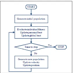
[image:32.612.218.469.399.649.2]is shown in Figure 2.7 below (Kohn,1998):
22 The first process of PSO is initialization where the initial swarm of
particles is generated. Each particle is initialized with random position and
velocity. Then, each particle will be evaluated for fitness value. Each time a fitness
value is calculated, it is compared against the previous best fitness value of the
whole swarm, and the personal best and global best positions are updated where
appropriate. If a stopping criterion is not met, the velocity and position are updated
to create a new swarm. The personal best and global best positions, as well as the
old velocity, are used in the velocity update. The process is repeated until a
stopping criterion is met.
2.7 Correlation
Correlation is widely used in digital signal processing because it is
easy to understand and implementation. Correlation can be defined as the degree
of similarity between two signals. If the two signals are identical, then the
correlation coefficient is 1. However, if the both signals are totally different, the
correlation coefficient becomes 0 and if both signals are identical but the phase is
shifted by exactly 180º (known as mirror), then the correlation coefficient is -1.
Correlation can be divided into two which are cross-correlation and
autocorrelation. When two independent signals are compared, it is known as
cross-correlation and when the same signal is compared to phase shifted copies of
itself, it is known as autocorrelation.
2.7.1 Cross-correlation
The cross-correlation is a very useful tool that investigates the degree
of association between two signals (Eialli,2004). An important use of the
23 function of the delay between them. The cross-correlation between ( ) and ( )
can be described by (Taghizahed,2000):
( ) ∫ ( ) ( ) (2.12)
Or
( ) ∫ ( ) ( ) (2.13)
Where:
T: The period of observation
( ): Always real-valued
The properties of cross-correlation are shows in Table 2.1 below:
Table 2.1: Properties of Cross-correlation function (Taghizahed,2000)
( ) s always a real valued function which may be positive or negative.
( ) may not necessarily have a maximum at m=0 nor ( ) an even
function.
( ) ( )
2.7.2 Autocorrelation
The autocorrelation is an operation that involves identical function
(Ljung,1998). Autocorrelation may be viewed as a measure as similarity, or
coherence, between a function ( ) and it is shifted version. Clearly, under no
24 But with increasing shift, it would be natural to expect the similarity and hence the
correlation between ( ) and its shifted version decrease. As the shift approaches
infinity, all traces of similarity will be vanishing and the autocorrelation decays to
zero.
Consider a random process ( ) (continues-time), the autocorrelation function is
written as below in equation (2.14) (Taghizahed,2000);
( ) ∫ ( ) ( ) (2.14)
Where:
T: The period of observation
( ): Always real-valued and an even function with a maximum value at τ=0
[image:35.612.137.550.483.705.2]The properties of autocorrelation are shows in Table 2.2 below:
Table 2.2: Properties of Autocorrelation function (Taghizahed,2000)
Autocorrelation Properties
Maximum value The magnitude of the autocorrelation function of a wide sense
stationary random process at lag m is upper bounded by its
value at lag m=0:
( ) | ( )|
Periodicity If the autocorrelation function of a WSS (Wide Sense
Stationary) random process is such that:
71 REFERENCE
Aly, Ayman A. (2011). PID Parameter Optimization Using Genetic Algorithm Technique for Electrohydraulic Servo Control System. Intelligent Control and Automation, 69-76.
Blondin, James. (2009). Particle Swarm Optimization: A Tutorial.
Chao-Ming Huang,Chi-Jen Huang,Ming-Li Wang. (2005). A Particle Swarm Optimization to Identifying The ARMAX Model for Short-term Load Forecasting. IEEE Transactions on Power System, 1126-1133.
Eialli, Taan S. (2004). Discrete Systems and Digital Signal Processing with MATLAB. New York: CRC Press.
Engelbrecht, A. P. (2006). Particle Swarm Optimization: Where does it belong? Proc,IEEE Swarm Intell,Swmp, 48-54.
Gautam, Bijaya. (2010). Spectral Estimation of Electroencephalogram Signal using ARMAX Model and Particle Swarm Optimization. Texas: Lamar University.
Gupta, S. a. (2014). Robust PID Tuning of Heat Exchanger System using Swarm Optimization Method. International Journal of Recent Technology of Engineering (IJRTE), 2277-3878.
Hannan, Dunsmuir, Deistler and H.Bierens. (1980). Estimation of Vector ARMAX Models. Journal of Multivariate Analysis, 275-295.
HE Shang Hong, LI Xuyu, Zhong Jue. (2002). Identification of ARMAX based on Genetic Algorithm. Trans. Nonferrous Met. Soc. China, 349-355.
Holland, John H. (1975). Adaptation in Natural and Artificial Systems: An
72 Ibrahim, Saifudin bin Mohamed. (2005). The PID Controller Design using
Genetic Algorithm. Toowoomba, Queensland: University of Southern Queensland.
Jacob Chi-Man Yiu, Shengwei Wang. (2007). Multiple ARMAX Modeling Scheme for Forecasting Air Conditioning System Performance. Energy Conversion and Management, 2276-2286.
James Kennedy and Russell Eberhart. (1995). Particle Swarm Optimization. In Proceedings of the IEEE International Conference on Neural Networks, Volume IV, 1942-1948.
James Kennedy, Russell C. Eberhart,Yuhui Shi. (2001). Swarm Intelligence. Morgan Kaufmann.
Jawa, Sara Natasha Ak. (2011). An ARMAX Model of QAD BDT 921 Heat Exchanger Identification. Batu Pahat: Universiti Tun Hussein Onn (UTHM).
Johansson, Rolf. (1993). System Modeling and Identification. Englewood Cliffs, New Jersey: Prentice-Hall.
Kachitvichyanukul, Voratas. (2012). Comparison of Three Evolutionary Algorithms: GA, PSO, and DE. Industrial Engineering & Management Systems, 215-223.
Kohn, Andre Fabio. (1998). Autocorrelation and Cross-Correlation Methods. Sao Paulo: University of Sao Paulo.
Ljung, Lennart. (1998). System Identification: Theory for the User. Englewood Cliffs,NJ: Pearson Education.
M.J. Jimenez, H. Madsen, K.K. Andersen. (2008). Identification of The Main Thermal Characteristics of Building Components Using MATLAB . Building and Environment, 170-180.
Maurice Stewart, Oran T. Lewis. (2011). Heat Exchanger Equipment Field Manual: Common Operating Problems and Practical Solutions. Waltham, USA: Gulf Professional Publishing.
Noor Adzmira binti Mustapha, T. M. (2011). General Polynomial Model to System Identification of Heat Exchanger Based on Hammerstein Wiener Model. UTHM.
73 Ramesh K. Sha, D.P. Sekulic. (2003). Fundamentals of Heat Exchanger Design.
New Jersey: John Wiley&Sons.
Raymond Chong, Shao Fen. (n.d.). Boiler Drum and Heat Exchanger Process Control Training System.
Sadik Kakac, H. L. (2012). Heat Exchangers: Selection, Rating, and Thermal Design (2nd ed.). CRC Press.
Taghizadeh, S.R. (2000). Digital signal Processing. London: University of North London.
Tatang Mulyana, Mohd Nor Mohd Than, Dirman Hanafi. (2009). A Discrete Time Model of Boiler Drum and Heat Exchanger QAD Model BDT 921.
International Conference of Instrumentation, Control & Automation, 154-159.
Tham, M.T. (1999). Dynamic Models for Controller Design. Newcastle: University of Newcastle.
Thulukkanam, Kuppan. (2000). Heat Exchanger Design handbook, Second Edition. Chennai, india: CRC Press.
Yamille del Valle,Ganesh Kumar Venayagamoorthy,Salman Mohagheghi,Jean-Carlos Hemandez,Ronald G. Harley. (2006). Particle Swarm Optimization: Basic Concepts, Variants and Applications in Power Systems. IEEE
Transactions on Evolutionary Computation, 171-193.