Neutral point inverter controller using h infinity techniques

NEUTRAL POINT INVERTER CONTROLLER USING H INFINITY TECHNIQUES

ALI OMAR .M ALSHARIF

A thesis report submitted in partial

fulfillment of the requirement for the award of the Degree of Master of Electrical and Electronic Engineering

Faculty of Electrical and Electronic Engineering Universiti Tun Hussien Onn Malaysia

ABSTRACT

ABSTRAK

2.1 Introduction 4

2.2 Three-Phase Inverter 4

2.2.1 Pulse Width Modulation 10

2.3 Three-level Neutral-point Inverter 11

2.3.1 Circuit Topology 11

2.4 Controller 12

2.4.1 Open-loop control systems 12

2.4.2 Closed-loop control systems 13

2.5 Controllers for neutral point application 15 TABLE OF CONTENT

TITLE i

ACKNOWLEDGEMENT iv

ABSTRACT v

ABSTRAK vi

TABLE OF CONTENT vii

LIST OF FIGURE x

LIST OF TABLE xiii

CHAPTER 1 INTRODUCTION 1

1.1 Project Background 1

1.2 Problem Statements 3

1.3 Project Objectives 3

1.4 Project Scopes 3

2.5.1 P Controller 15

2.5.2 PD Controller 16

2.5.3 PI Controller 16

2.5.4 PID Controller 17

2.5.5 P-Resonant controller 19

2.6 H∞ control 21

2.7 H∞ controller and Its operational methodology 23

CHAPTER 3 METHODOLOGY 24

3.1 Introduction 24

3.2 System block diagram 24

3.3 Project flow chart 26

3.4 Modelling of the neutral line circuit 27

3.5 Realizations of the Plant P 31

3.6 K∞ controller

34

3.7 Function of K∞ controller 35

CHAPTER 4 RESULT AND ANALYSIS 36

4.1 Introduction 36

4.2 Circuit Simulation for Neutral point three phase inverter

36

4.2.1 Open Loop Neutral point three phase inverter By Using Simulink

37

4.3 Analysis for Neutral point three phase inverter 37 4.3.1 Analysis for Open Loop Neutral point three phase inverter

38

by using Simulink

4.4 Analysis for Neutral point three phase inverter with H∞ controller with a reference of zero amperes.

41

4.5 Analysis for Neutral point three phase inverter with H ∞ controller with a reference 2A.

43

4.6 Analysis for Neutral point three phase inverter with H∞ controller with a reference 5A.

45

CHAPTER 5 CONCLUSION AND RECOMMENDATION 48

5.1 conclusion 48

5-2 Recommendation 49

REFERENCES 50

LIST OF FIGURE

Figure Title Page

Fig 2.1 Three-phase inverter network 5

Fig 2.2a Split DC- link neutral connection 6

Fig 2.2b A fourth-leg neutral connection used with three dimensional space-vector modulations

7

Fig 2.2c The neutral line circuit under consideration .The combination of Fig 2.2a and 2.2b the actively balanced split DC link

7

Fig 2.3 General block diagram 8

Fig 2.4: Voltage Source Inverter (VSI) 8

Fig 2.5 Current Source Inverter (CSI) 8

Fig 2.6 Three-Phase Half Bridge Inverter 9

Fig 2.7 Three-phase Full-Bridge Inverter 9

Fig 2.8 Conventional three-phase Voltage-Source Inverter 10

Fig 2.9 Pulse Width Modulation 11

Fig 2.10 The schematic diagram of a conventional three-level neutral-point clamped voltage source inverter using the IGBT switches

12

Fig 2.11: Open loop control system 13

Fig 2.12 Block diagram of a closed loop control system 14

Fig 2.13 Closed loop process control system 15

Fig 2.14 basic control systems 15

Fig 2.15 PI controller block diagram 17

Fig 2.16 PID control logic 19

Fig 2.17 P-Resonant controllers 20

Fig 2.18 Frequency response characteristic of the open loop P+ resonant Controller

21

Fig 2.19 The standard H∞ optimal control problem 22

Fig 2.20 Standard H∞ control problem for DC-AC inverter 23

Fig 3.2 Project flow chart 26 Fig 3.3 Flowchart of designing three phase inverter circuit using

MATLAB Simulink and neutral point.

27

Fig 3.4 T fi v 29 Fig 3.5 The neutral line circuit under consideration. 29

Fig 3.6 The block diagram of the neutral leg 30

Fig 3.7 Proposed of the H∞ control problem for neutral point control 31 Fig 4.1 Simulation open loop neutral point three phase inverter by

using MATLAB software

37

Fig 4.2 output current for open loop circuit neutral point three phase inverter

38

Fig 4.3 output voltage for open loop circuit neutral point three phase inverter

38

Fig 4.5 Capacitor current for open loop circuit neutral point three phase inverter.

39

Fig 4.5 Inductor current for open loop circuit neutral point three phase inverter

39

Fig 4.6 Simulation neutral point three phase inverter with H∞ controller 40 Fig 4.7 output current for close loop circuit neutral point three phase

inverter

41

Fig 4.8 output voltage for close loop circuit neutral point three phase inverter

41

Fig 4.9 Capacitor current for closed loop neutral point three phase inverter circuit.

42

Fig 4.10 Inductor current for closed loop neutral point three phase inverter circuit

42

Fig 4.11 Output current for close loop circuit neutral point three phase inverter.

43

Fig 4.12 Output voltage close loop circuit neutral point three phase inverter.

43

Fig 4.13 Capacitor current for closed loop neutral point three phase inverter circuit.

44

inverter circuit.

Fig 4.15 Output current for close loop circuit neutral point three phase inverter

45

Fig 4.16 Output voltage for close loop circuit neutral point three phase inverter

45

Fig 4.17 Capacitor current for closed loop neutral point three phase inverter circuit

46

Fig 4.18 Inductor current for closed loop neutral point three phase inverter circuit

LIST OF TABLE

Table Title Page

2.1 Effects of Coefficients 19

2.2 Advantage of PID 19

CHAPTER I

INTRODUCTION

1.1 Project Background

A power inverter, or inverter, is an electrical power converter that changes direct current(DC) to alternating current (AC); the converted AC can be at any required voltage and frequency with the use of appropriate transformers, switching, and control circuits [1].

Inverters can be broadly classified into two types, voltage source and current source inverters. A voltage fed inverter (VFI) or more generally a voltage–source inverter (VSI) is one in which the DC source has small or negligible impedance. The voltage at the input terminals is constant. A current–source inverter (CSI) is fed with adjustable current from the DC source of high impedance that is from a constant DC source. A voltage source inverter employing thyristors as switches, some type of forced commutation is required, while the (VSI) made up of using GTOs, power transistors, power MOSFETs or IGBTs, self-commutation with base or gate drive signals for their controlled turn-on and turn-off.

Since the neutral point of an electrical supply system is often connected to neutral, under certain conditions, a conductor used to connect to a system neutral is also used for grounding of equipment and structures. Current carried on a grounding conductor can result in objectionable or dangerous voltages appearing on equipment enclosures, so the installation of grounding conductors and neutral conductors is carefully defined in electrical regulations. Where a neutral conductor is used also to connect equipment enclosures to earth, care must be taken that the neutral conductor never rises to a high voltage with respect to local ground.

1.2 Problem Statements

The neutral line is usually needed to provide a current path for possible balanced loads and the traditional six-switch inverter must be supplemented with a neutral connection. If the neutral point of a four-wire system is not well balanced, then the neutral-point voltage may deviate severely from the real midpoint of the DC source. This deviation of the neutral point may result in an unbalanced or variable output voltage, the presence of the DC component, larger neutral current or even more serious problems. Thus, the generation of a balanced neutral point in a simple and effective manner has become an important issue. These issues are mainly due to the lack of control and feedback.

1.3 Project Objectives

The objectives of this study are formulated as follows:

1) To design the H∞ control strategy that is suitable for neutral point inverter. 2) To analyse the output from the inverter with and without the controller. 3) To maintain a stable and balanced neutral point, which makes as small as

possible while maintaining the stability of the system.

1.4 Project Scopes

This project based on the following scopes:

1) Modelling of three phase DC-AC inverter with neutral point connection and controller strategyis simulated using MATLAB Simulink software. 2) Using intelligent technique as controller to improve power inverter for

system.

CHAPTER II

LITERATURE REVIEW

2.1 Introduction

In this chapter generally given introduction about some of types of controls and neutral point of three phase inverter and it also focus on controller. The basic components and their detailed functions will be introduced and discussed.

2.2 Three-Phase Inverter

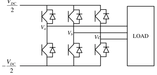
The principles for the physical layout of three phase inverters, also known as voltage-source converters (VSC:s) are shown in Figure 2.1 The bridge is connected to the DC link, whose voltage is raw material in the creation of the three phase output voltage. The link voltage is from now on called DC link. The mid potential of the DC-link is defined as neutral.

LOAD Va

Vb

Vc

2

DC

V

2

DC

V



Figure 2.1: Three-phase inverter network.

Between the two poles of the DC link, the three half-bridges are connected. Each half bridge has two power electronic switches. By switching them, between fully conducting and fully blocking, the potentials of each half-bridge ( , , , with

respect to the mid potential of the DC link, can attain ± /2.

The neutral current usually makes the neutral point shift. The shift of the neutral point may result in unbalanced variable output voltage, DC component in the output, larger neutral current or even more serious problems. The neutral line is usually needed on the AC side of the converter to provide a current path for the zero-sequence current components.

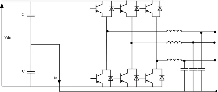
A straightforward way to provide the neutral point is to use two capacitors shown in Figure (2.2a), in parallel with large balancing resistors. Such a configuration is called a split DC link. Since the neutral current flows through the capacitors, very high capacitance is needed to make the voltage ripple on the capacitors small. Another drawback is that the neutral point usually drifts and becomes non-balanced, in particular, when the neutral current has a DC component. Hence, this topology is not suitable for DC-AC converters which supply power to possibly unbalanced consumers or to the grid. Since the neutral current in Active power filters does not have a DC component and the fundamental component is relatively small, the split DC link is widely used in Active power filters. There are three different circuit topologies have been widely used to generate a neutral point. The most popular topology is a split DC link, shown in Figure (2.2a), with the neutral point clamped at half of the DC link voltage. Since the neutral current flows through capacitors, high capacitance is necessary. Moreover, the neutral point usually shifts following capacitors and switches differences. To improve performance of the split DC link topology, different neutral point balancing strategies are reported, usually using redundant states of the Space Vector Pulse Width Modulation (SVPWM).

Vdc

In C

C

Vdc Ln+Rn

In C

Figure 2.2b: A fourth-leg neutral connection used with three dimensional space-vector modulations [4].

Vdc

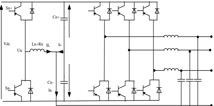
Sn- Sn+

Ln+Rn IL

In Ic

Cn-Cn+

Un

Figure 2.2c: The combination of Fig (2.2a and 2.2b), The Actively balanced split DC link [4].

According to the value of the load connected at the output so as to provide constant rated output.

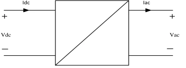
The DC to AC converters more often known as inverters, depending on the kind of the source of feeding and the related topology of the power circuit, are classified as voltage source inverters (VSI) and current source inverters (CSI). The following Figure (2.4) and Figure (2.5) illustrates the types of inverter.

Idc Iac

Vdc Vac

Figure 2.3: General block diagram Idc

Iac

Vdc Load Voltage

C DC LINK

Figure 2.4: Voltage Source Inverter (VSI)

Idc

I LOAD

Vdc Load Current

I DC L

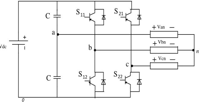
The three-phase counterparts of the single-phase half and the full bridge voltage source inverters are shown in Figures 2.6 and 2.7, Single-phase (VSI) covered low-range power applications and three-phase (VSI) covered medium to high power applications. The main purpose of these topologies is to provide a three-phase voltage supply, where the can be controlled amplitude, three-phase and frequency of the voltages can be controlled. The three-phase DC-AC voltage source inverters are widely used in motor drives, Active filters and unified power flow controllers in power systems and uninterrupted power supplies to generate controllable frequency. AC voltage magnitudes using various pulse width modulation (PWM) strategies. Standard of three-phase inverter shown in Figure 2.7 has six switches the switching of that depends on the scheme of modulation. Usually the input DC is obtained from a single-phase or three phase utility power supply through a diode-bridge rectifier and LC or C filter.

Vdc

Vcn Vbn Van

n

S ₁₂

S S

S 11 21 22 0 C C a b c

Figure 2.6: Three-Phase Half-Bridge Inverter

Vdc

Vcn Vbn Van

n

S ₂₂

S S

S 21 31 32 0 S S 12 11 a b c

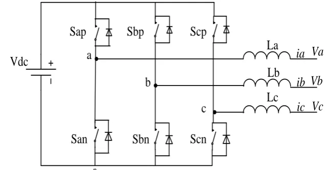
Three-Phase DC-AC inverter is commonly used in industry. There are many applications in industry that used this type of DC-AC conversion in order to operate. The types of inverters that are used to make sure all those applications operate have different types. Here are several types of three-phase inverter that are used in industry. Figure 2.8 shows a conventional three-phase voltage-source inverter VSI [9].

n

Sap Sbp Scp

San Sbn Scn

p ia ib ic La Lb Lc Va Vb Vc a b c Vdc

Figure 2.8: Conventional three-phase Voltage Source Inverter

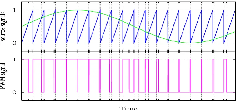
2.2.1 Pulse Width Modulation

In electronic power converters and motors, PWM is used extensively as a means of powering alternating current (AC) devices with an available direct current (DC) source or for advanced DC-AC conversion. Variation of duty cycle in the PWM signal to provide a DC voltage across the load in a specific pattern will appear to the load as an AC signal, or can control the speed of motors that would otherwise run only at full speed or off. The pattern at which the duty cycle of a PWM signal varies can be created through simple analog components, a digital microcontroller, or specific PWM integrated circuits.

tooth or triangular wave at a frequency significantly greater than the reference. When the carrier signal exceeds the reference, the comparator output signal is at one state, and when the reference is at a higher voltage, the output is at its second state. This process is shown in Figure 2.9 with the triangular carrier wave in red, sinusoidal reference wave in blue, and modulated and unmodulated sine pulses [20].

Figure 2.9: Pulse Width Modulation

2.3 Three-level Neutral-point Inverter

In order to provide the data base to modulation strategy proposed for the three-level-output-stage matrix converter, the three-level neutral point- clamped voltage source inverter technology from the operating principles to the related modulation diagram. The neutral-point balancing problem of the three-level neutral-point-clamped voltage supply inverter and associated control methods are also discussed.

2.3.1 Circuit Topology

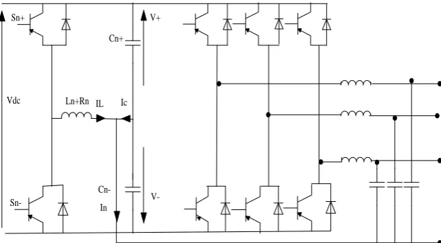
in Figure 2.10, the NPC VSI is supplied by two series-connected capacitors (C1 and C2), where both capacitors are charged to an equal potential of VDC, with the DC-link middle point ‘ ’ as a zero DC voltage neutral point. Each phase leg of the NPC VSI consists of four series-connected switching devices and two clamping diodes. These diodes clamp the middle switches’ potential to the DC-link point ‘ ’ [11].

Vdc

Sn- Sn+

Ln+Rn IL

In Ic

V+

Cn-Cn+

V-

Figure 2.10: The schematic diagram of a conventional three-level neutral-point clamped voltage source inverter using the IGBT switches

2.4 Controller

There are essentially two categories of control systems: open-loop and closed-loop. Both maintain a chosen variable at a selected level with different levels of success.

2.4.1 Open-loop control systems

structure of an open-loop control system. A few examples of open-loop control systems are bread toasters, ovens, washing machines and water sprinkler systems.

Figure 2.11: Open loop control system [13].

Open-loop control systems are in general relatively simple in design and inexpensive. However, require frequent operator intervention. Under many circumstances pre-set values become incorrect due to the parameter they are controlling changing in some way, and so they need resetting. The pre-set value often needs a high level of skill or judgement to set it correctly. In cases where the consequences of the system not controlling the parameter as desired are serious, such as the level of a hazardous liquid in a tank overflowing, open-loop systems are not suitable[19].

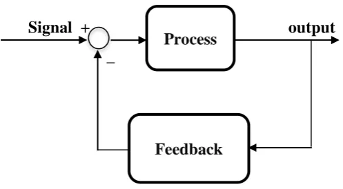
2.4.2 Closed-loop control systems

Signal + output

_

Figure 2.12: Block diagram of a closed loop control system

Feedback can be divided into positive feedback and negative feedback. Positive feedback causes the new output to deviate from the present command status. For example, an amplifier is put next to a microphone, so the input volume will keep increasing, resulting in a very high output volume. Negative feedback directs the new output towards the present command status, so as to allow more sophisticated control. For example, a driver has to steer continuously to keep his car on the right track. Most modern appliances and machinery are equipped with closed loop control systems.

An advantage of the closed-loop control system is the fact that the use of feedback makes the system response relatively insensitive to external disturbances (e.g. temperature and pressure) and internal variations in system parameters (e.g. Component tolerances) which are not known or predicted [18].

In closed-loop control systems the difference between the actual output and the desired output is feedback to the controller to meet desired system output. Often this difference, known as the error signal is amplified and fed into the controller. Figure 2.13 shows the general structure of a closed-loop feedback control system. A few examples of feedback control systems are elevators, thermostats, and the cruise control in automobiles.

Process

Figure 2.13: Closed loop process control system [13].

2.5 Controllers for neutral point application

Control systems are basically based on the feedback information from the main system. These systems are usually required to regulate and rectify the input of the system with respect to the desired output. The fundamental control system setup is depicted in Figure 2.14.

R e U Y +

_

Figure 2.14: basic control systems

2.5.1 P Controller

In general it can be said that P controller cannot stabilize higher order processes. For

_{order processes, the meaning of processes with one energy storage, a large}

increase in gain can be tolerated. Proportional controller can stabilize only _order

unstable process. Changing controller gain K can change closed loop system. A large Controller

C(s)

gain controller will result in control system with small steady state error, faster dynamics, phase margin and smaller amplitude.

When P controller is used, there will be a need to have a large gain to improve steady state error. Stable systems do not have problems when the gain is large; such systems are energy storage (1st order capacitive systems) systems. Constant steady state error can be accepted with such processes, and then P control can be used. Small steady state errors can be accepted if sensor will give measured value with error or if importance of measured value is not significant.

2.5.2 PD Controller

PD mode is used when prediction of the error can improve control or when it is necessary to stabilize the system.

To avoid effects of the sudden change of the reference input that will cause sudden change in the value of error signal. Sudden change in error signal will cause sudden change in control output. To avoid that it is suitable to design D mode to be proportional to the change of the output variable.

PD controller is often used in control of moving objects such as flying and

underwater vehicles, ships, rockets etc.

( (2.1)

2.5.3 PI Controller

However, introducing integral mode has a negative effect on speed of the response and overall stability of the system. Thus, the PI controller will not increase the speed of response. It can be expected since PI controller does not have means to predict what will happen with the error in near future. This problem can be solved by introducing derivative mode which has ability to predict what will happen with the error in near future and thus to decrease a reaction time of the controller. PI controllers are very often used in industry, especially when speed of the response is not an issue.

A control without D mode is used when fast response of the system is not required, large disturbances and noise are present during operation of the process, there is only one energy storage in process (capacitive or inductive), and there are large transport delays in the system.

( (2.2)

Integral (I)

Proportional (P) + plant Pla

R(S) + + C(S)

_

Figure 2.15: PI controller block diagram

2.5.4 PID Controller

This control theory is one of the classic controls, which is simple, easy to implement, and cheap. If assumed that the Actual velocity of the car can be measured, the error

G(S)

𝐾

can be calculated easily by targeting actual velocity. Most control theories use the error to track the reference, especially PID control uses this error multiplied by proportional, derivative, and integral gain to track the target. In this case, proportional gain is P, derivative gain is D, and integral gain is I, called "PID controller". P gain usually influences how fast the systems can response, D is used to reduce the magnitude of the overshoot, and I-controller used to eliminate the steady-state error. But there is no optimal solution in this controller. For example, if PID is combined together, the combination of PID gains affects the system response not affect independently. Thus there is no solution to find the optimal gain so usually PID gains are specified by tuning. As a result of this feature, PID controller is mostly used in Linear-Time Invariant (LTI) system and Single-Input Single-Output (SISO) system not in non-linear and complex Multi-Input Multi-Output (MIMO) system. To tune the system response, usually the system specification is set at the first. Then each gain is tuned to satisfy the system response specification defined such as per cent overshoot, rising time, settling time, and so on.

A PID controller has proportional, integral and derivative terms that can be represented in transfer function form as [12].

( (2.3)

PID controller has all the necessary dynamics: fast reaction with any change of the controller input (D mode), increase in control signal to lead error towards zero (I mode) and suitable action inside control error area to delete oscillations (P mode). The control PID is used when dealing with higher order capacitive processes when their dynamic is not similar to the dynamics of an integrator.

+

R (t) + u (t) y (t) + +

_

Figure 2.16: PID control logic [12].

Table 2.1: Effects of coefficients

Table 2.2: Advantages of PID

2.5.5 P-Resonant controller

This controller aims to get a good reference tracking and to reduce the output voltage harmonic distortion when the inverter feeds linear and nonlinear loads.The parameter Speed of

response

stability Accuracy

Increasing K Increases Deteriorate Improves

Increasing KI Decreases Deteriorate Improves

Increasing KD Increases Improves No impact

Response Rise time Overshoot Settling time S-S error

Decrease Increase NT Decrease

Decrease Increase Increase Eliminate

NT Decrease Decrease NT

𝐾

𝐾

𝐾

resonant controller is a generalized PI controller that is able to control not only DC but also AC variables, Figure 2.17 shows the structure of the resonant controller [15].

V(s) + + Y(s) -

Figure 2.17: P-Resonant controllers

In addition to a forward integrator there is another integrator in the feedback loop. The transfer function is given by

Figure 2.18 shows bode diagram of the resonant at a resonance frequency of 50Hz. At 50Hz there is an infinite open loop gain and thus it is able to eliminate the steady state error at this frequency. If ω would be zero the resonant controller has the same structure as the well-known PI controller [16].

𝑆 𝜔2

𝐾𝐼

𝐾_𝑃

Figure 2.18: Frequency response characteristic of the open loop P+ resonant Controller

2.6 control

is used in control theory to synthesize controllers, achieving stabilization with guaranteed performance. To use methods, a control designer expresses the control problem as a mathematical optimization problem and then finds the controller that solves this. techniques have the advantage over classical control techniques in that they are readily applicable to problems involving multivariable systems with cross-coupling between channels.

External input W Z External output

U

y

Figure 2.19: The standard optimal control problem

From the Figure 2.19,

[

_{] ( [}

_]

Suppose P(s) can be partitioned as follows

P(s) = [ 11( 12(

21( 22( ] (2.6)

From equation (2.5) and (2.6),

Z = 11w + 12u (2.7)

y = ₂₁w + ₂₂u (2.8)

Then with the feedback law u = K(s) y can eliminate u and y

Z = [ ₁₁ + ₁₂K (I − ₂₂K 1 ₂₁w (2.9)

= 1(P, K) w (2.10)

P(s)

2.7 H∞ controller and Its Operational Methodology

From Figure 2.20, G is the DC-AC inverter, K is the transfer function of H∞ controller, is a stable weight function, the vector represents references current and y represents output voltage.

The standard problem of H∞ controller is to find K that stabilizes the plant P minimizing the infinity norm of the close-loop transfer function

By using MIXSYN- Mixed-Sensitivity-Loop-Shaping. This MATLAB function computes a controller K that minimizes the H∞ norm of the closed-loop transfer function.

PLANT ̃

PLANT

+

-

d

y

Controller

Figure 2.20: Standard H∞ control problem for DC-AC inverter.

𝜔

_

G

K

𝑉𝐷𝑐

2

CHAPTER III

METHODOLOGY

3.1 Introduction

The chapter describes about the methodological procedures which have been followed during the implication of this study. It familiarises about the introduction of the topology of the basic simulative setup. The fundamental system design is represented in terms of block diagrams and the systematic procedure of the project implementation is presented. The chapter concludes by illustrating the modelling of neutral point circuitry as it has been simulated using MATLAB/Simulink.

3.2 System block diagram

Figure 3.1: System block diagram. DC-AC Inverter DC

Source Load

𝐻

PWM +I ref

REFERENCE:

[1] Holmes, D. Grahame, and Thomas A. Lipo. Pulse width modulation for power converters: principles and prACtice. Vol. 18. Wiley-IEEE Press, 2003.

[2] Lipo, Thomas A. Vector control and dynamics of AC drives. Vol. 41. Oxford University Press, USA, 1996.

[3] Tomas Hornik and Qing-Chang Zhong.” current control strategy for the neutral point of a three-phase inverter” 2011 50th IEEE Conference on Decision and Control and European Control Conference (CDC-ECC) Orlando, FL, USA, December 12-15, 2011.

[4] Q.-C. Zhong, Senior Member, IEEE, J. Liang, Member, IEEE, G. Weiss, Member, IEEE, Chunmei Feng, and Timothy C. Green, Senior Member, IEEE” H∞ Control of the Neutral Pointin Four-Wire Three-Phase DC–AC Converters” IEEE TRANSACTIONS ON INDUSTRIAL ELECTRONICS, VOL. 53, NO. 5, OCTOBER 2006.

[5] Zhang, Wenping, Xiao Li, Chengrui Du, Xiaotian Wu, Guoqiao Shen, and Dehong Xu. "Study on neutral-point voltage balance of level NPC inverter in 3-phase 4-wire system." In Power Electronics for Distributed Generation Systems (PEDG), 2010 2nd IEEE International Symposium on, pp. 878-882. IEEE, 2010. [6] Yazdani, Amirnaser, and Reza Iravani. Voltage-Sourced Converters in Power Systems. Wiley, 2010.

[7] Tomas Hornik, Member, IEEE, and Qing-Chang Zhong, Senior Member, IEEE. Parallel PI Voltage–H∞ Current Controller for the Neutral Point of a Three-Phase Inverter. IEEE TRANSACTIONS ON INDUSTRIAL ELECTRONICS, VOL. 60, NO. 4, APRIL 2013.

[8] Lipo, Thomas A. Vector control and dynamics of AC drives. Vol. 41. Oxford University Press, USA, 1996.

[9] William S. Levine, Robert T. Reichert An Introduction to H, Control System Design-Honolulu, Hawaii December 1990.

[11] Three-level Neutral-point-clamped Matrix Converter Topology. Meng Yeong Lee. University of Nottingham for the degree of Doctor of Philosophy,

March 2009.

[12] Hornik, Tomas. Power quality in microgrids. Diss. The University of Liverpool, 2010.

[13] Dorf, Richard C. and Robert H. Bishop, Modern Control Systems, 9th ed., Prentice–Hall Inc., New Jersey-07458, USA, 2001, Chapters 1, 5, pp. 1-23, pp. [14] Chuen Chien Lee (1990), Fuzzy Logic in Control Systems: FuzzyLogic Controller Part I, llXr TransACtions On Systtms. Man, Ani,

[15] R. Teodorescu, F. Blaabjerg, U. Borup, and M. Liserre. A new control structure for grid-connected lcl pv inverters with zero steady-state error and selective harmonic compensation. In Applied Power Electronics Conference and Exposition, 2004. APEC ’04. Nineteenth Annual IEEE, volume 1, pages 580–586 Vol.1, 2004. [16] Xiaoming Yuan, W. Merk, H. Stemmer, and J. Alleging. Stationary-frame generalized integrators for current control of ACtive power filters with zero steady-state error for current harmonics of concern under unbalanced and distorted operating conditions. Industry Applications, IEEE TransACtions on, 38(2):523–532, Mar/Apr 2002.

[17]Ljung, Lennart. System identification. John Wiley & Sons, Inc., 1999.

[18] Aström, Karl Johan, and Richard M. Murray. FeedbACk systems: an introduction for scientists and engineers. Princeton university press, 2010.

[19] Hart, John K. Automatic control program creation using concurrent Evolutionary Computing. Diss. Bournemouth University, 2004.