Recursive Estimation for Continuous Time Stochastic Volatility Models Using the Milstein Approximation

http://dx.doi.org/10.4236/jmf.2013.33036 Published Online August 2013 (http://www.scirp.org/journal/jmf)

Recursive Estimation for Continuous Time Stochastic

Volatility Models Using the Milstein Approximation

Theodoro Koulis1, Alexander Paseka2, Aerambamoorthy Thavaneswaran1 1

Department of Statistics, University of Manitoba, Winnipeg, Canada 2

Department of Accounting and Finance, University of Manitoba, Winnipeg, Canada Email: [email protected], [email protected], [email protected]

Received May 11, 2013; revised June 14, 2013; accepted June 28, 2013

Copyright © 2013 Theodoro Koulis et al. This is an open access article distributed under the Creative Commons Attribution License, which permits unrestricted use, distribution, and reproduction in any medium, provided the original work is properly cited.

ABSTRACT

Optimal as well as recursive parameter estimation for semimartingales had been studied in [1,2]. Recently, there has been a growing interest in modelling volatility of the observed process by nonlinear stochastic processes [3]. In this paper, we study the recursive estimates for various classes of discretely sampled continuous time stochastic volatility models using the Milstein approximation. We provide closed form expressions for the recursive estimates for recently proposed stochastic volatility models. We also give an example of computation of the term structure of zero rates in an incomplete information environment. In this case, learning about an unobserved state variable is done jointly with the valuation procedure.

Keywords: Recursive Estimation; Diffusion Processes; Interest Rate Models; Milstein Approximation

1. Introduction

In the last three decades, semimartingales have received considerable attention with the emphasis being placed on state space models. From an econometric standpoint, time-varying volatility models have been widely devel- oped, recognizing that the volatility and the correlation of assets change over time (see for example [4]). State space models in which the conditional mean of the ob- served process is modeled as a stochastic process are useful in parameter estimation. For example, stochastic volatility models are widely employed to estimate vola- tility parameters [3,5].

In [2], the estimating function approach was used for the recursive parameter estimation in models with semi- martingales. In [1,6,7], the estimating function method was used for the estimation of state space models in the Bayesian setup. Parameter estimates obtained in [2] in- volve the evaluation of the stochastic integrals based on the observation of the complete path of the observed process. However, for continuous time models, it is more appropriate to study parameter estimates based on dis- cretely observed data. In order to study the inference for diffusion processes based on discretely observed data, one has to approximate the continuous time diffusion by a discrete process. For some interest rate models (e.g. Vasicek, Cox-Ingersoll-Ross), discrete time approxima-

tion has been used to study parameter estimation (see [8,9] and the references therein).

Recursive estimation expresses the estimate of the pa-

rameter at time t1 in terms of the parameter at time

t and an adjustment based on the observation at time

1



t . Continuous time volatility models have been stud-

ied in [10]. However, the recursive parameter estimation based on discrete approximation have not been studied in the literature.

In most realistic situations, the diffusion cannot be observed continuously, so discrete time approximations to stochastic integrals or a direct approach using discrete time observations is required. For extended versions of the Cox-Ingersoll-Ross (CIR) model (see [11]), closed form expressions for the first four conditional moments cannot be obtained easily by using Ito’s formula, as was done for the non-extended CIR model (see [9]). Recently, [11] uses the Milstein approximation [12] to obtain the first two conditional moments of a diffusion. For dif- fusion models with a finite number of parameters, [9] uses the Milstein approximation to obtain the first four conditional moments and to construct the optimal esti- mating functions for the Vasicek model of the form

 

dy_t _tdt_tdW t ,

drawbacks of this one-factor model is that it is not in general possible to calibrate it so that it fits the presently observed term structure. For example, [13, p. 171] points out that for the above Vasicek model, which depends on

three parameters,  ,  , and  , it is not possible to

choose values of those parameters so that the entire ob- served term structure of interest rates is fitted exactly by the model. To solve the problem, Kennedy proposes to allow time-varying parameters in the drift term of the Vasicek model.

Consider a diffusion process given by the time-ho- mogeneous stochastic differential equation of the form





d



, _t



d

 

dy_t a ,y_t

W t

t

t b W t

α β y

d

 



d d

(1)

where and are the drift and diffusion functions,

respectively, and is the standard Brownian mo-

tion. A special case of (1) is the Brownian motion with constant drift and diffusion coefficients:

a b



 

,

y  t W t

where  > 0. In this case, the conditional distribution of

t given is a normal with mean

y y0 y yt and

variance 2_t

. If we consider the geometric Brownian motion given by

 

dy_t y t_td y W t_td ,

with > 0, then log



yt



becomes a Brownian motion

with drift with     2 2 and  

 

. In this case,

the conditional distribution of log yt given log

 

y0

 

log y

 is also normal. The CIR process can be re-

parameterized to the following form:



1 2



 

t t

y   y

1 2

t t

y   y

d d y W t_td .

dW t



t

 

 

 

Extended versions of the CIR process model have been proposed for modelling interest rate processes. For example, some consider the constant elasticity of vari- ance process of the form





2

 

1

d dt y_t

or the nonlinear drift diffusion process (see [14]) given by



 

4

3

3

t t

y  y

2 1

4

d d

d .

t t

y y t

W t

  

 



1 2

1 2

t t

y   y

 

 

 

For more general extended models, the diffusion is a

function of the observation t and hence, closed form

expressions of the conditional distributions, as well as closed form expressions for the conditional moments cannot be easily obtained by solving differential equa- tions obtained by repeated application of Itô’s formula. However, the Milstein approximation can be used to ob- tain the first four conditional moments.

y

If we consider a discretisation in small intervals of

time titi1h, then the Milstein approximation ap-

plied to (1) produces











 





1 1 1

1 1

2

, ,

1

, , 1

2

i i i i

i i i

t t t t

t y t t ,

i

t

y y a y h b y h

b y b y h





  

 

  

  

α β

β β (2)

where y

b b

y

 



 _and

_

_{0,1 , i.i.d.}

i

t N

 



Unlike the Euler approximation for diffusion processes, the Milstein method in (2) gives a non-Gaussian time series model for

1

i i

t t

y y_ . The distribution implied by

the Milstein approximation is a mixture of a normal and chi-square distribution. Moreover, for the extended CIR model and for more general diffusion processes, Ito’s approximation cannot be used to obtain closed form ex- pressions for the first four conditional moments. In this paper, first we use the Milstein approximation to discre- tise the continuous time diffusion processes and then study the recursive estimates of latent state variables. We also show how the proposed method can be used to de- rive zero coupon bond prices in the incomplete informa- tion environment. In this case, the valuation exercise and the recursive estimation (learning) of the unobserved state variable are performed simultaneously by market participants.

2. State Space Models

In order to construct an optimal recursive estimate for non-normal stochastic volatility models, we start with the following discrete time example.Let the discrete-time

state space model of the observed process

 

yt and the

state process

 

t be given by:









2

1 1 1

2

1 1

1

1

t t t t

t t t t

y A az b z

B c d



   

  

  1

   

    (3)

where A B a b c, , , , and are positive constants, and

possibly measurable with respect to the

d

 -field

generated by the observations of



y t





s

y up to and in-

cluding time t. In addition,

 

zt and



t



are two

standard Gaussian sequences of identically distributed

random variables with Corr



z_t,_t



. The following

lemma will be used to prove our main Theorem.

Lemma 1 Assume that Z1N

 

0,1 and Z2 N

 

0,1

with Corr



Z Z1, 2



. Then



2 2 1, 2

Z Z



2

Corr  .

Proof 1 It follows from the theorem on Normal corre-

lation that the conditional expectation and conditional variance of Z1 given Z2 are give by

1 2 2

E Z Z_  _ Z and VarZ Z1 2  



1 2



.









2 2 2 2

1 2 2 1 2

2 2 2 4

2 2

2 2

1

1 3 1 2

E Z Z E Z E Z Z

E Z   Z

2 .                  _   _     

Hence, the correlation between 2

1

Z and 2

2

Z is given

as



_{2 2}



12 22 ₂ 1 2

1

Corr , .

4 E Z Z

Z Z 

  

 

 

The following theorem establishes the recursive esti- mation for the state space model (3).

Theorem 1 Given the state space model (3), and the class of all estimators of the form:





1 1

ˆ ˆ ˆ _{ˆ ,}

t B t G yt t A t

_    _  

the Gt, which minimizes the mean-square error,





2

1 1 ˆ 1

y

t E t t

     

 t ,

is given by





2 2 2

2 ˆ _. 2 t t t

AB ac bd

G

A a b

  



 



 

Moreover, the mean-square error is given as













2

2 2 1

2 2 2

ˆ ₂

ˆ _{2 2} ˆ ₂

t t t

t t

B AG c d

G a b G ac bd

 

 

    

    .

1

Proof 2 The difference t1ˆt





2

.  is given by





























2

1 1 1 1

2

1 1

1

2

1 1 1

ˆ ˆ ₁

ˆ 1

ˆ

1 1

t t t t t t

t t t t t

t t t t

t t t t t

B c d

G A az b z A

B AG c

d aG z bG z

                                        

Squaring the above expression, taking expectations, and using the results of Lemma 1 it follows that the

con-ditional mean-square error at t1 is given by













2 _{2 2 2 2 2}

1 2 2

2 2 .

t t t t

t

B AG c d G a b

G ac bd

 

 

      

 

Differentiating t1 with respect to and setting

the first derivative to zero, we have t G













2 2 2 2

2 2 0.

t t t 2

A B AG G a b

ac bd



 

   

  

Solving for Gt, we obtain





2 2 2

2 2 ˆ 2 2 t t t

AB ac b

G

A a b

         d 1

Corollary 1 Let the state space model be of the form

1 1, 1 .

t t t t t t

y A z  B  

where

 

zt and

 

t are two sequences of independ-

ent and identically distributed random variables having

mean zero and variance 2

z

 and 2



 , respectively. In

the class of estimates of the form:





1 1 1

ˆ ˆ ˆ _{ˆ ,}

t B t G yt t A t

_  _  _  

the Gt which minimizes the mean-square error



ˆ



y t E t t F

  _  _t _

 

is given by

2 2

ˆ t _.

t t z BA G A     

In addition, the mean-square error is given as





2

2 2 2

1 ˆ ˆ .

t B G At t  Gt z

_      

Proof 3 The result follows from Theorem 1 by setting z

a= , b=, c=d=0, and =0.

3. General Model

In the continuous-time setting, consider the general state space model of the form

 

 

 

 





 

1 2

d d d

d d , d

t t t t

t t t t t

y A y t y W t

B y t y W t

 

   

 

 

,

where W t1

 

and W t2

 

are two uncorrelated standard

Brownian motions. If we consider a discretisation in

small intervals of time titi1h, , then the

Milstein approximation gives a non-Gaussian discrete state-space model of the form:

0,1,

i 

 

 

   



 

 



 



1 1 1 1 1 1 2 2 1 , 2 1 , , 2

i i i i i i

i i i

i i i i

i i i i i

t t t t t t

t y t t

t t t t

t t t t t

y y A y h y hz

h

y y z

B y h y h

h

y _ y

                          _{ } 



1 , i t      (4)

where y

y



 



 and y

     

 _{, and}





_and

i t

z

 

i t



are two independent standard Gaussian sequences of in- dependent and identically distributed random variables.

We relate the discretised model (4) to the discrete-time model (3) by letting

1

1 _{i i}

t t t

y_ y_ y ,

1

1 _i

t t

1

1 i

t t

z_ z_ , and t1ti₁. In addition, we have

 

ti

A A y , a

 

yt_i h ,

   

2 ti y ti

h

b  y  y ,

 

yti 1

B B h_, c

 

yt_i h,



,

 

i i

t t

y

 ,



2 ti ti

h

d   y    , and 0. It now follows

from Theorem 1 that the recursive estimator is of the form

 

t B yt h

    

 



 





1 1

ˆ ₁ ˆ ˆ ˆ _,

i t G yt t A yti h

      t

where

 

 



   

2 2 i i t t A y y  

 

2 2 2

1 ˆ _, 1 2 i i i i

t t t

t

t t y t

B y h

G

A y h h y y

    _       _  _   

and the mean-square error is given as

 





 





 





   

2 2 1 2

2 2 2

ˆ 1

1 _{ˆ ˆ}

, ,

2

1

ˆ _.

2

i i i

i i

i i i

t t t t

t t

t y t

A y G y h

y

h h y y

                      2 2 2 2 i i t t t t t t

B y h

h y

G y

 



 

Example 1 (Klebaner’s Model) [15] considers a state space model in which the conditional mean of the ob- served diffusion process is modeled by the Black-Scholes process (see [16]) and given by:

 

 

1

2

2

d d d ,

d d d

2

t t

t t t

y t W t

t W           _  _ 

  t ,

where and are two independent standard

Brownian motions. In this case, the Milstein approxima- tion leads to

 

1

W t W t2

 





1 1 1 1 2 2 2 , 2 1 . 2

i i i i

i i i i i

i i

t t t t

t t t t t

t t

y y h hz

h h h   1                    _  _     

 (0.5)

We relate (5) to the discrete-time model (3) by letting

1

1 _{i i}

t t t

y_  y_ y ,

1

1 _i

t t

 _ , zt1 zt_i₁, and t1ti1.

Also, we put Ah, a h, , b0

2

1

2

B _ _ _h_

   

 , cti h and

2

2 ti

h

d   . It

now follows from Theorem 1 that the recursive estimator is of the form





2

1 1

ˆ ₁ ˆ ˆ _,

2

t h t G yt h

 _ˆ t t _       _         where





2 1 2 ˆ _, 1 t t t h G h                    

and the mean-square error is given as

2 2

1

2 2 2 4 2 2

ˆ 1

2

1

ˆ ˆ ˆ _.

2

i i

t t

t t t

h hG

h h G h

 t              _     _         

Example 2 (Hull and White Model) [17] proposed a stochastic volatility model in which the conditional va- riance of the observed diffusion process is modeled by a Black-Scholes process and given by:

 

 

1 2 2 2

2

d d d

d d d

t t t t

t t t

y y t y W t

a t b W t

         , .

where W t1

 

and W t2

 

are two correlated standard

Brownian motions with E_dW t₁

 

dW t₂

 

_dt. We

use Ito’s formula to obtain d_t:

 

2

2

d d

2 8 2

t t t

a b b

t W





 _  _  

_{} d t

To simplify the Milstein approximation, we treat the

coefficient on dW t₁

 

as a function of only . In this

case, the Milstein approximation leads to t y













1 1 1 1 2 2 2 2 1 1 , 2 1 1 2 8

i i i i i i i i i

i i i i i i

t t t t t t t t t

t t t t t t

y y y h y hz y h z

b b

h h h

                         1 1 .   i (6)

We relate (6) to the discrete-time model (3) by letting

1

1 _{i i}

t t t t

y y_ y y h, t1t_i₁, zt1zti1, t1ti1.

Also, we put A0 ,

i i t t

a y h , 1 2

2 ti ti

b  y h ,



1



B _h ,

2 ti

b

c h and 2

8 ti

h

d b . It now

follows from Theorem 1 that the recursive estimator is of the form





1 1

ˆ ₁ ˆ _,

t h t G y

   ˆ

and the mean-square error is given as





2 2 2 2 4 2 1

2 2 2 2 2

ˆ ˆ

1

4 32

1

ˆ ˆ ₁ ˆ ˆ ˆ ₁ ˆ

2

t t t t

t t t t t t t t

b h

h h b

h

y hG h h b y G b

                    _  _ _ 

    4 .

  

When correlation  0, the model simplifies to









1

2 2

2 2 4

1

ˆ _0, ˆ ₁ ˆ_,

ˆ ˆ

1

4 32

t t t

t t t

G h

b h

h h b

     2 . t              

Example 3 (CIR Model) Consider the CIR model for observed process yt given by





1

 

dytk tyt dt y W ttd ,

and the state process t follows a diffusion process of

the form

 





2

 

dt B yt tdt yt,t dW t ,

 

 

1 2

d d

E_ W t W t _0.

In this case, the Milstein approximation for yt and

t

 leads to





 

 



 



1 1 1 1 1 1 2 2 2 1 1 , 4 1 , , 2

i i i i i i

i

i i i i

i i i i i

t t t t t t

t

t t t t

t t t t t

y y ky k h y hz

h z

B y h y h

h

y _ y

                          _{ } 

  1 ,



i

t

 (7)

respectively.

We relate (7) to the discrete-time model (3) by letting

i

1

1 i i

t t t t

y_  y_ y ky , t1ti₁, zt1 zti1, t1ti1,

and  0. Also, we put Akh,

i t

a y h,

2

1 4

b  h , 1

 

,

i t

B B y h_

 

i t

c y h and



,

 

,



i i

t t

y



2 ti ti

h

d   y   

t

. It now follows from Theorem

1 that the recursive estimator is of the form

 





1 1

ˆ ₁ ˆ ˆ ˆ _,

i

t B yt h t Gt yt kh

  _ _    

where

 

2 2 2

1 ˆ _, 1 8 t t t t t

k B y h

G

k h y

             _  _  

and the mean-square error is given as

 





 

   

2 2 1 2

2 2 2 2

ˆ 1

1

ˆ ˆ ˆ

, ,

2 8

i

t t t t t

t t t t t t

B y h khG y h

h

y _ y hG y

                  _{ }   

4. Bond Valuation with Recursive Learning

under Milstein Approximation

We now present the computation of a zero coupon bond price in the setting of a two-factor CIR model. In two- factor models, in general, bond yields are deterministic (and usually affine) functions of two factors. There are at least two reasons for why two-factor (or even multi-fac- tor) models are more preferable to single-factor models. First, the empirical difficulties of fitting the shape of the term structure of zero rates and their volatilities and the variation of interest rate spreads in single-factor models are well known. Second, there are institutional restric- tions on the behavior of interest rates that mandate more factors than one. Central banks tend to target certain lev- els (or ranges) of interest rates. These levels themselves may change over time as economic conditions change. As an example we consider a variant of the two-factor CIR model presented in [18]. The model defines the short rate as a CIR process with long-run mean (also known as central tendency) being itself a CIR process:









d d

d d

t r t t r t r

t t

r r t r

t z d , d , t z                  

where E



dzrdz_



=0. The Milstein approximation is

readily available:

















2 2 2 2 1 , 4 1 , 4 r

t h t r t t r t r r

t h t t t

r r r h r h h

h h  h

                                  (8)

and E r   0. Note that the new state variable

processes are no longer normal. Rather, they are a mix- ture of normal and chi-squared random variables.

Because investors do not observe t, the task of pric-

ing a zero coupon bond is a two-stage exercise. First,

investors estimate the latent central tendency process, ˆ_t.

For that purpose, we assume they use the rule described in Theorem 1, so that





ˆ







ˆt h ˆt  ˆt h G rt t h rt r ˆt r ht ,

           



2 2 2 ˆ _, 8 r t t r r t r t

h G h r               

 h

and

2

h







2

2 2 2 2 2 ˆ _ˆ 1 8 ˆ _. 8

t h r t t t

r

t r t

h hG h h

G h r h

This last term simplifies to







2 ₂



2 2

ˆ ˆ

1 2 3

ˆ .

8

t h r t t r t

t

h hG G h

h h



 



    



 

    

 

 _  _

 

where is the time price of a zero coupon bond

with periods remaining until maturity. The complete

information version of this model is affine, and the solu- tion for a bond price in the complete information case is available in continuous time. Here, we can start with dis- crete-time SDF

n t B

n

t









2

1 2

ln mt h rt r ht r r.

Second, investors value the bond conditional on the

pair



r_t,ˆ_t . Thus, investors’ problem is the joint prob-

lem of estimation of the latent state process and simulta- neous valuation of the bond.

h

     



     (10)

Finding SDF parameter restrictions requires the knowl- edge of the following integral of an exponential-quadratic

function of a standard normal variable, :

The fundamental valuation principle in asset pricing states that if there is no arbitrage, then there exists a posi- tive pricing kernel (also called stochastic discount factor (SDF)) such that the following condition is satisfied by

any h-period return on any asset at any time:





2

2 1 1

exp exp

2 1 2 1 2

t

t t t

t t

E     

 

 

   _{ }

  _{   } (11)

with transversality condition t< 1 2. The condition that





1.

t t h t h

E m R  (9)

the expectation of an -period SDF has to give us the

-period short rate allows us to find SDF coefficient restrictions:

h h

In our example we are interested in an -period re-

turn on a zero coupon default-free bond, h

n n h t h Bt t h

R_ B_  ,

 













2





1 2

ln Bth =r ht = ln Etexp lnmt h  = ln Etexp  rt  r ht r  h r  .

  _{ }  _     _

Using the fundamental pricing Equation (9), the SDF expression (10), and the expression for the expectation of the exponential-quadratic function of the standard normal variable in (11), we have

must have



2



1

ln 1 2 ,

2 h

   

 

2 1

2 2

ln

1 1

ln .

2 1 2 1 2

h

t t

t t

B r h

r h r

h h

  

 

 

 

   _ _

 

 

(12)

2 1

2

1

1 .

2 1 2 h

h  



 

 _  _



 

Inserting SDF (10) into the pricing Equation (9), we obtain the following expression for the price of a zero-

coupon bond maturing at time T (let



Tt



hN):

For SDF (10) to be consistent with restriction (12), we







   



1

2

, , 2 , 1 , , 1 2 , 1

0

exp exp .

N T

t t t h t h t h T h T t t t nh t t nh r t n h r t n h

n

E m m m B N E r  r h h 



         



  

     _{ }    _

  _{ }









By definition, the yield on this bond is given by

 



   



1

2

1 , , 1 2 , 1

=0

1 1

ln ln exp .

N

T T

t t t t nh t t nh r t n h r t n h

n

y B N E r r h h

T t T t      



     

   

  _  _        

 

 







Unfortunately, the learning implications of the model render the final bond expression non-affine in the state variables. The expectation above, however, can be easily computed using Monte Carlo integration.

When constructing the term structure of interest rates

we make maturities, , range from one year to 10 years.

The discretisation time step, , is kept constant at

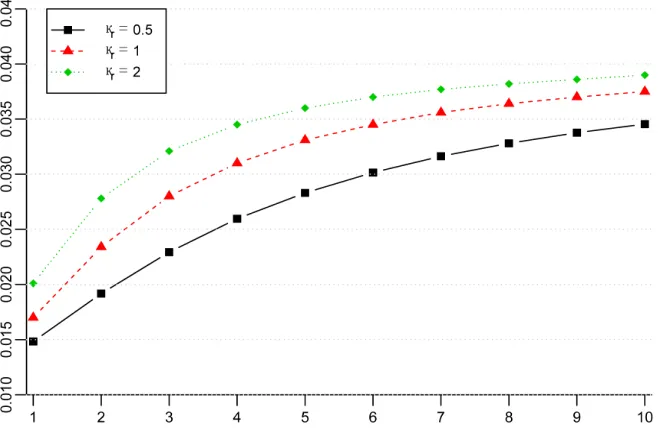
of a year. As a base case for our simulations we take the following parameter values. We choose the speed of mean reversion in both the short rate and the

central tendency to be

T

h 1/500

2.0

r 

   , so that they are

consistent with high persistence of the state variables.

E.g., for  r 2.0, the persistence of the non-Gaussian

AR(1) short rate process in (8) is equal to

r

1 h0.996. Both r and  have virtually iden-

tical impact on the term structure of zero yields1. This

influence, however, is strong as we might expect. Intui- tively, larger speed of mean reversion pulls the state

variables faster to the long run mean, . The result is

1

that all yields are larger with the intermediate yields be- ing affected the most, which increases the concavity of

the term structure as represented in Figure 1.

The shape of the term structure strongly depends on the relative position of the current short rate with respect

to the long run mean of the central tendency, 2. Our

model produces rich patterns of the term structure similar to non-discretised CIR models. If the short rate is below the mean, the term structure is upward-sloping, otherwise, it is inverted. For our numerical results we set the long

run mean of the central tendency at in the base

case. The level of

0.01

 has a strong effect on both the lev-

els and the curvature of the term structure, with the latter

being affected the most by  than any other parameter

of the model (see Figure 2).

Our numerical simulations show that, interestingly, the instantaneous volatilities of both the short rate and the central tendency are largely irrelevant for the shape and level of the term structure. We start with the base case

values of the volatilities given by r  0.01

0%

. As an example, the yields on a -year and 10 -year zeros in

the base case are and 3.9 , respectively. If

we increase

1 2.01%

r

 substantially to, say, 0.1, the corre-

sponding new yields are identical to those obtained with

base case parameters. Likewise, if we increase _ from

0.01 to 0.1, we do not see any change in any of the yields3.

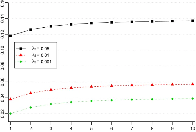
The base case risk premiums are   1 0.02 and

2 0.001

  . Zero yields are largely insensitive to the

value of 1. However, the second risk premium, which

is the loading on the non-Gaussian component in the SDF, has strong influence on the term structure. This non-Gaussian risk premium affects zero rates of all ma-turities in the same way leading to parallel shifts in the yield curve. Even though the shape of the term structure is largely not affected, the yields are very sensitive to the

level of the second risk premium. E.g., a change in 2

from the base case level of 0.001 to 0.05 adds about 980

basis points to yields of all maturities as shown in Figure

3.

5. Conclusion

[image:7.595.135.465.379.594.2]

Recently, it has been demonstrated (see [19]) that the diffusion process can be well approximated by the Mil- stein approximation rather than the Euler approximation.

Figure 1. Term structure as a function of the speed of mean reverison in the short rate. We use base parameters presented in the text to generate the term structure of zero rates. The underlying model is the discretized version of a continuous-time Cox-Ingersoll-Ross (CIR) model with central tendency of the short rate also following a CIR process. We use the Milstein discretization scheme. The curves represent the mean yields over 10,000 Monte Carlo iterations. The time step in the Milstein scheme is 1/500 of a year. The speed of mean reversion parameter, ranges from 0.5 to 2. In our simulations, we assume that both the short rate and the central tendency start at 0.01. We also assume that the posterior variance of the central tendency estimate, λt, starts at the level of two instantaneous standard deviations of the central tendency,

r

κ

t η t

γ = 2σ η per year.

2_{In our simulations, we assume that both the short rate and the central tendency start at 0.01. We also assume that the posterior variance of the central} tendency estimate, t, starts at the level of two instantaneous standard deviations of the central tendency, t, i.e., t2  t per year.

[image:8.595.131.464.83.312.2]

Figure 2. Term structure as a function of the central tendency of the short rate. We use base parameters presented in the text to generate the term structure of zero rates. The underlying model is the discretized version of a continuous-time Cox-Ingersoll-Ross (CIR) model with central tendency of the short rate also following a CIR process. We use the Milstein discretization scheme. The curves represent the mean yields over 10,000 Monte Carlo iterations. The time step in the Milstein scheme is 1/500 of a year. The long run mean of the central tendency, θ, ranges from 0.1 to 0.4. In our simulations, we assume that both the short rate and the central tendency start at 0.01. We also assume that the posterior variance of the central tendency estimate, λt, starts at the level of two instantaneous standard deviations of the central tendency, γt= 2ση ηt per

year.

Figure 3. Term structure as a function of the second rsik premium, λ2. We use base parameters presented in the text to

generate the term structure of zero rates. The underlying model is the discretized version of a continuous-time Cox-Ingersoll- Ross (CIR) model with central tendency of the short rate also following a CIR process. We use the Milstein discretization scheme. The curves represent the mean yields over 10,000 Monte Carlo iterations. The time step in the Milstein scheme is 1/500 of a year. The non-Gaussian risk premium, λ2, ranges from 0.5 to 2. In our simulations, we assume that both the short

rate and the central tendency start at 0.01. We also assume that the posterior variance of the central tendency estimate, λt,

[image:8.595.128.465.425.652.2]

In this paper, we study the recursive estimates for various classes of discretely sampled continuous time stochastic volatility models using the Milstein approximation. We also provide an example of joint valuation of a zero- coupon bond and learning about an underlying state variable under incomplete information environment.

REFERENCES

[1] A. Thavaneswaran and M. E. Thompson, “A Criterion for Filtering in Semimartingale Models,” Stochastic Proc- esses and Their Applications, Vol. 28, No. 2, 1988, pp. 259-265. doi:10.1016/0304-4149(88)90099-3

[2] A. Thavaneswaran and M. E. Thompson, “Optimal Esti- mation for Semimartingales,” Journal of Applied Prob- ability, Vol. 23, No. 2, 1986, pp. 409-417.

doi:10.2307/3214183

[3] S. Taylor, “Asset Price Dynamics, Volatility, and Predic- tion,” Princeton University Press, Princeton, 2011. [4] S. L. Heston and S. Nandi, “A Closed-Form GARCH

Option Valuation Model,” The Review of Financial Stud- ies, Vol. 13, No. 3, 2000, pp. 585-625.

doi:10.1093/rfs/13.3.585

[5] H. Kawakatsu, “Specification and Estimation of Discrete time Quadratic Stochastic Volatility Models,” Journal of Empirical Finance, Vol. 14, No. 3, 2007, pp. 424-442. doi:10.1016/j.jempfin.2006.07.001

[6] U. V. Naik-Nimbalkar and M. B. Rajarshi, “Filtering and Smoothing via Estimating Functions,” Journal of the American Statistical Association, Vol. 90, No. 429, 1995, pp. 301-306. doi:10.1080/01621459.1995.10476513 [7] M. E. Thompson and A. Thavaneswaran, “Filtering via

Estimating Functions,” Applied Mathematics Letters, Vol. 12, No. 5, 1999, pp. 61-67.

doi:10.1016/S0893-9659(99)00058-0

[8] A. Thavaneswaran, Y. Liang and N. Ravishanker, “Infer- ence for Diffusion Processes Using Combined Estimating Functions,” Sri Lankan Journal of Applied Statistics, Vol.

12, No. 1, 2012, pp. 145-160.

[9] T. Koulis and A. Thavaneswaran, “Inference for Interest Rate Models Using Milstein’s Approximation,” Journal of Mathematical Finance, Vol. 3, No. 1, 2013, pp. 110- 118. doi:10.4236/jmf.2013.31010

[10] H. Gong and A. Thavaneswaran, “Recursive Estimation for Continuous Time Stochastic Volatility Models,” Ap- plied Mathematics Letters, Vol. 22, No. 11, 2009, pp. 1770-1774. doi:10.1016/j.aml.2009.06.014

[11] M. Jeong and J. Y. Park, “Asymptotic Theory of Maxi- mum Likelihood Estimator for Diffusion Model,” Work- ing Paper, Indiana University, 2010.

[12] P. E. Kloeden and E. Platen, “Numerical Solution of Sto- chastic Differential Equations,” Applications of Mathe- matics, Vol. 23, 1992, in press.

doi:10.1007/978-3-662-12616-5

[13] D. Kennedy, “Stochastic Financial Models,” Financial Mathematics Series, Chapman & Hall/CRC, London, 2010.

[14] Y. Ait-Sahalia, “Testing Continuous-Time Models of the Spot Interest Rate,” Review of Financial Studies, Vol. 9, No. 2, 1996, pp. 385-426. doi:10.1093/rfs/9.2.385

[15] F. Klebaner, “Introduction to Stochastic Calculus with Applications,” Imperial College Press, London, 2005. doi:10.1142/p386

[16] F. Black and M. S. Scholes, “The Pricing of Options and Corporate Liabilities,” Journal of Political Economy, Vol. 81, No. 3, 1973, pp. 637-654. doi:10.1086/260062 [17] J. C. Hull and A. D. White, “The Pricing of Options on

Assets with Stochastic Volatilities,” Journal of Finance, Vol. 42, No. 2, 1987, pp. 281-300.

doi:10.1111/j.1540-6261.1987.tb02568.x

[18] P. Balduzzi, S. R. Das and S. Foresi, “The Central Ten- dency: A Second Factor in Bond Yields,” The Review of Economics and Statistics, Vol. 80, No. 1, 1998, pp. 62-72. doi:10.1162/003465398557339