Testing Finitary Probabilistic Processes

(1)

Testing Finitary Probabilistic Processes: DRAFT

Yuxin Deng

1 ∗

, Rob van Glabbeek

2,4

, Matthew Hennessy

3†

& Carroll Morgan

4‡ 1

_{Shanghai Jiao Tong University, China}

2

_{NICTA, Sydney, Australia}

3

_{Trinity College Dublin, Ireland}

4

_{University of New South Wales, Sydney, Australia}

January 11, 2010

Abstract

This paper provides modal- and relational characterisations of may- and must-testing preorders for recursive CSP processes with divergence, featuring probabilistic as well as nondeterministic choice. May testing is characterised in terms of simulation, and must testing in terms of failure simulation. To this end we develop weak transitions between probabilistic processes, elaborate their topological properties, and capture divergence in terms of partial distributions.

1 Introduction

It has long been a challenge for theoretical computer scientists to provide a firm mathematical foundation for process-description languages that incorporate both nondeterministic and probabilistic behaviour in such a way that processes are semantically distinguished just when they can be told apart by some notion of testing.

In our earlier work [3, 2] a semantic theory was developed for one particular language with these characteristics, a finite process calculus calledpCSP: nondeterminism is present in the form of the standard choice operators inherited from CSP [9], that isP ⊓QandP 2_Q, while probabilistic behaviour is added via a new choice operatorPp⊕Q in whichP is chosen with probabilitypandQwith probability1−p. The intensional behaviour of apCSPprocess is given in terms of a probabilistic labelled transition system [23, 3], or pLTS, a generalisation of labelled transition systems [19]. In a pLTS the result of performing an action in a given state results in a probability distribution over states, rather than a single state; thus the relationss −→α tin an LTS are replaced by relationss −→α ∆, with∆a distribution. ClosedpCSPexpressionsPare interpreted as probability distributions[P℄in the associated pLTS. Our

semantic theory [3, 2] naturally generalises the two preorders of standard testing theory [5] topCSP:

• P ⊑pmay Qindicates thatQis at least as good asP from the point of view of possibly passing probabilistic tests; and

• P ⊑pmustQindicates instead thatQis at least as good asPfrom the point of view of guaranteeing the passing of probabilistic tests.

The most significant result of [2] was an alternative characterisation of these preorders as particular forms of co-inductively defined simulation relations,⊑Sand⊑FS, over the underlying pLTS. We also provided a characterisation

in terms of a modal logic.

(3)

τ τ

a

1/2 1/2

a

τ τ _τ

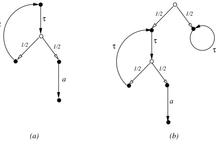
[image:3.612.197.421.20.168.2]

(a) (b)

Figure 1: The pLTSs of processesQ1andQ2

The simulation relations⊑S and⊑FS in [2] were defined in terms of weak transitions=⇒ˆτ between distributions,

obtained as the transitive closure of a relation−→ˆτ between distributions that allows one part of a distribution to make aτ-move with the other part remaining in place. This definition is however inadequate for processes that can do an unbounded number ofτ-steps. The problem is highlighted by the processQ1 = recx.(τ.x 1

2⊕ a.0)illustrated in Figure 1(a). ProcessQ1is indistinguishable, using tests, from the simple processa.0: we haveQ1 ≃pmay a.0and

Q1≃pmusta.0. This is because the processQ1will eventually perform the actionawith probability 1. However, the

action[a.0℄

a

−→[0℄can not be simulated by a corresponding move[Q1℄

ˆ

τ

=⇒_−→a _{. No matter which distribution}_∆

we obtain from executing a finite sequence of internal moves[Q1℄

ˆ

τ

=⇒ ∆, still part of it is unable to subsequently perform the actiona.

To address this problem we propose a new relation ∆ =⇒ Θ, that indicates thatΘcan be derived from∆ by performing an unbounded sequence of internal moves; we callΘa weak derivative of∆. For example[a.0℄will turn

out to be a weak derivative of[Q1℄,[Q1℄=⇒[a.0℄, via the infinite sequence of internal moves

[Q1℄

τ −→[Q11

2⊕a.0

℄

τ −→[Q1 1

22⊕a.0

℄

τ

−→. . .[Q1 1

2n⊕a.0℄

τ −→. . . .

One of our contributions here is the significant use of “sub distributions” that sum to no more than one [10, 18]. For example, the empty subdistributionεelegantly represents the chaotic behaviour of processes that in CSP and in must-testing semantics is tantamount to divergence, because we haveε_−→α _ε_{for any action}_α_{, and a process like}_rec_{x. x}

that diverges via an infiniteτpath gives rise to the weak transitionrecx. x=⇒ε. So the processQ2=Q11

2⊕recx. x illustrated in Figure 1(b) will enable the weak transition[Q2℄ =⇒

1

2[a.0℄, where intuitively the latter is a proper

subdistribution mapping the statea.0to the probability 1₂. Our weak transition relation=⇒can be regarded as an extension of the weak hyper-transition from [16] to partial distributions; the latter, although defined in a very different way, can be represented in terms of ours by requiring weak derivatives to be total distributions.

We end this introduction with a brief glimpse at our proof strategy. In [2] the characterisations for finitepCSP processes were obtained using a probabilistic extension of the Hennessy-Milner logic [19]. Moving to recursive processes, we know that process behaviour can be captured by a finite modal logic only if the underlying LTS is finitely branching, or at least image-finite [19]. Thus to take advantage of a finite probabilistic HML we need a property of pLTSs corresponding to finite branching in LTSs: this is topological compactness, whose relevance we now sketch.

Subdistributions over (derivatives of) finitarypCSPprocesses inherit the standard (complete) Euclidean metric. One of our key results is that

Theorem 1.1 For every finitarypCSPprocessP, the set{∆ | [P℄=⇒∆}is convex and compact.

Indeed, using techniques from Markov Decision Theory [21] we can show that the potentially uncountable set{∆ |

(4)

P ::= S | Pp⊕P

S ::= 0 | x∈Var | a.P | P ⊓P | S2_S _| _S_|_A_S _| _rec_{x. P}

Figure 2: Syntax ofpCSP

This key result allows an inductive characterisation of the simulation preorders⊑Sand⊑FS, here defined using

our novel weak derivation relation=⇒. We first construct a sequence of approximations⊑k

S fork ≥ 0and, using

Theorem 1.1, we prove

Theorem 1.2 For every finitarypCSPprocessP, and for everyk ≥ 0, the set{∆ | [P℄ ⊑

k

S ∆}is convex and

compact.

This in turn enables us to use the Finite Intersection Property of compact sets to prove

Theorem 1.3 For finitarypCSPprocesses we haveP ⊑S QiffP ⊑kS Qfor allk≥0.

Our main characterisation results can then be obtained by extending the probabilistic modal logic used in [2], so that for example

• it characterises⊑k

Sfor everyk≥0, and therefore it also characterises⊑S

• every probabilistic modal formula can be captured by a may-test.

Similar results accrue for must testing and the new failure simulation preorder⊑FS: details are given in Section 8.

2 The language

pCSP

LetActbe a set of visible actions which a process can perform, and letVarbe an infinite set of variables. The language pCSPis then given by the two-sorted syntax in Figure 2. It is essentially the finite language of [2, 3], to which has been added the recursive constructrecx. P in whichxis a variable andP a term. Intuitivelyrecx. P represents the solution of the fixed-point equationx =P. The notions of free and bound variables are standard, as is that of the substitution of terms for free occurrences of variables (with renaming if necessary). ByQ[x7→P]we mean the result of substituting the termPfor the variablexinQ.

We writepCSPfor the set of closed terms defined by this grammar, thepCSPprocesses, andsCSPfor its subset ofpCSPstates: the sub-sortSabove.

The processP p⊕ Q, for0≤p≤1, represents a probabilistic choice betweenP andQ: with probabilitypit will act likeP and with probability1−pit will act like Q.1 Any process is a probabilistic combination of state-based processes built by repeated application of the operatorp⊕. The state-based processes have a CSP-like syntax, involving the stopped process0, action prefixinga. fora∈Act, internal- and external choices⊓and2, and a parallel composition|AforA⊆Act.

The process P ⊓ Qwill first do a so-called internal actionτ6∈Act, choosing nondeterministically betweenP andQ. Therefore⊓, likea. , acts as a guard, in the sense that it converts any process arguments into a state-based process. The same applies torecx. Pas, following CSP [20], our recursion construct performs an internal action when unfolding. As our testing semantics will abstract from internal actions, theseτ-steps are harmless and merely simplify the semantics.

The processs 2 _ton the other hand does not perform actions itself but rather allows its arguments to proceed, disabling one argument as soon as the other has done a visible action. In order for this process to start from a state rather than a probability distribution of states, we require its arguments to be state-based as well; the same requirement applies to|A.

1_{In our semantics we have}

[P0⊕Q℄=[Q℄and[P1⊕Q℄=[P℄, so without limitation of generality we could have required that0<p<1.

(5)

Finally, the expressions |A t, whereA ⊆ Act, represents processess andt running in parallel. They may

synchronise by performing the same action fromAsimultaneously; such a synchronisation results inτ. In additions andtmay independently do any action from(Act\A)∪ {τ}.

Although formally the operators2_and_|_A _{can only be applied to state-based processes, informally we use} ex-pressions of the formP 2_Q_and_P _|_A _Q_{, where}_P _and_Q_{are not state-based, as syntactic sugar for expressions in} the above syntax obtained by distributing2and|Aoverp⊕. Thus for examples 2 (t1p⊕t2)abbreviates the term

(s2_t₁₎_p_⊕_(s2_t₂₎.

The full language of CSP [1, 9, 20] has many more operators; we have simply chosen a representative selection, and have added probabilistic choice. Our parallel operator is not a CSP primitive, but it can easily be expressed in terms of them — in particularP |A Q = (PkAQ)\A, wherekA and\Aare the parallel composition and hiding

operators of [20]. It can also be expressed in terms of the parallel composition, renaming and restriction operators of CCS. We have chosen this (non-associative) operator for convenience in defining the application of tests to processes. As usual we may elide0; the prefixing operatora. binds stronger than any binary operator; and precedence between binary operators is indicated via brackets or spacing. We will also sometimes use indexed binary operators, such asL

i∈Ipi·PiwithPi∈Ipi= 1and allpi >0, andei∈IPi, for some finite index setI.

Our language is interpreted as a probabilistic labelled transition system [3, 2]. Essentially the same model has appeared in the literature under different names such as NP-systems [11], probabilistic processes [12], simple prob-abilistic automata [22], probprob-abilistic transition systems [13] etc. Furthermore, there are strong structural similarities with Markov Decision Processes [21, 4].

We now fix some notation. A (discrete) probability subdistribution over a setSis a function∆ :S →[0,1]with

P

s∈S∆(s)≤ 1; the support of such a∆is⌈∆⌉:= {s∈S | ∆(s) >0}, and its mass|∆|is

P

s∈⌈∆⌉∆(s). A subdistribution is a (total, or full) distribution if|∆|= 1. The point distributionsassigns probability1tosand0to all other elements ofS, so that⌈s⌉={s}. WithD(S)we denote the set of subdistributions overS, and withD1(S)

its subset of full distributions.

Let{∆k |k∈K}be a set of subdistributions, possibly infinite. ThenPk∈K∆k is the real-valued function in

S→Rdefined by(P

k∈K∆k)(s) :=Pk∈K∆k(s). This is a partial operation on subdistributions because for some

statesthe sum of∆k(s)might exceed1. If the index set is finite, say{1..n}, we often write∆1+. . .+ ∆n. For

pa real number from[0,1]we usep·∆to denote the subdistribution given by(p·∆)(s) :=p·∆(s). Finally we use εto denote the everywhere-zero subdistribution that thus has empty support. These operations on subdistributions do not readily adapt themselves to distributions; yet if thatP

k∈Kpk = 1for some collection ofpk ≥0, and the∆k are

distributions, then so isP

k∈Kpk·∆k. In general when0≤p≤1we writexp⊕yforp·x+ (1−p)·ywhere that makes sense, so that for example∆1p⊕∆2is always defined, and is full if∆1and∆2are.

The expected valueP

s∈S∆(s)·f(s)over a distribution∆of a bounded non-negative functionf to the reals or

tuples of them is written Exp_∆(f), and the image of a distribution∆through a functionf is written Img_f(∆)— the latter is the distribution over the range offgiven by Img_f(∆)(t) :=P

f(s)=t∆(s).

Definition 2.1 A probabilistic labelled transition system (pLTS) is a triplehS, L,→i, where (i) Sis a set of states,

(ii) Lis a set of transition labels,

(iii) relation→is a subset ofS×L× D1(S).

A (non-probabilistic) labelled transition system (LTS) may be viewed as a degenerate pLTS — one in which only point distributions are used. As with LTSs, we writes−→α ∆for(s, α,∆)∈ →, as well ass−→α for∃∆ :s−→α ∆ ands→for∃α:s −→α . A pLTS is finitely branching if the set{hα,∆i |s−→α ∆, α∈L}is finite for all statess; if moreoverSis finite, then the pLTS is finitary. A pLTS is deterministic if for each statesand labelα, there is at most one distribution∆withs−→α ∆.

The operational semantics ofpCSPis defined by a particular pLTShsCSP,Actτ,→iin whichsCSPis the set of

states andActτ :=Act∪ {τ}is the set of transition labels; we letarange overActandαoverActτ. We interpret

pCSPprocessesPas distributions[P℄∈ D1(sCSP)via the function[ ℄:pCSP→ D1(sCSP)defined by

(6)

(action)

a.P −→a [P℄

(recursion)

recx. P −→τ [P[x7→recx. P]℄

(int.l)

P ⊓Q_−→τ

[P℄

(int.r)

P ⊓Q_−→τ

[Q℄

(ext.l)

s1−→a ∆

s12s2−→a ∆

(ext.r)

s2−→a ∆

s12s2−→a ∆

(ext.i.l)

s1−→τ ∆

s12s2−→τ ∆2s2

(ext.i.r)

s2−→τ ∆

s12s2−→τ s12∆

(par.l)

s1−→α ∆

s1|As2−→α ∆|As2

α6∈A

(par.r)

s2−→α ∆

s1|As2−→α s1|A∆

α6∈A

(par.i)

s1−→a ∆1, s2−→a ∆2

s1|As2−→τ ∆1|A∆2

a∈A

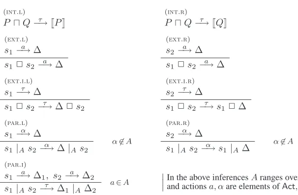
[image:6.612.97.400.48.247.2]

In the above inferencesAranges over subsets ofAct, and actionsa, αare elements ofAct,Actτ respectively.

Figure 3: Operational semantics ofpCSP

The transition relation → is defined in Figure 3. This is a very slight extension of the rules we used earlier [3, 2] for finite processes: one new rule is required to interpret recursive processes. All rules are very similar to the standard ones used to interpret CSP as a labelled transition system [20], but are modified so that the result of an action is a distribution. The rules for external choice and parallel composition use an obvious notation for distributing an operator over a distribution; for example∆2_s_{represents the distribution given by}

(∆2_{s)(t) =}

(

∆(s′₎ _if_t₌_s′ ₂_s

0 otherwise.

We sometimes writeτ.P forP⊓P, thus givingτ.P −→τ [P℄.

The set of states reachable from a subdistribution ∆ is the smallest set that contains⌈∆⌉and is closed under transitions, meaning that if some statesis reachable ands −→α Θthen every state in⌈Θ⌉is reachable as well. We graphically depict the operational semantics of apCSPexpressionPby drawing the part of the pLTS reachable from

[P℄as a directed graph with states represented by filled nodes•and distributions by open nodes◦. For any states

and distribution∆withs_−→α _∆_{we draw an edge from}_s_to_∆_{labelled with}_α_{; and for any distribution}_∆_{and state}_s

in⌈∆⌉, the support of∆, we draw an edge from∆toslabelled with∆(s). Sometimes we partially unfold this graph by drawing the same nodes multiple times; in doing so, all outgoing edges of a given instance of a node are always drawn, but not necessarily all incoming edges.

Note that for eachP∈pCSPthe distribution[P℄has finite support. Moreover, our pLTS is finitely branching in

the sense that for each states∈sCSPthere are only finitely many pairs(α,∆)∈Actτ× D1(sCSP))withs−→α ∆.

In spite of[P℄’s finite support, and the finite branching of our pLTS, it is possible for there to be infinitely many states

reachable from[P℄; when there are only finitely many, thenPis said to be finitary [4].

(7)

3 Lifted transitions, and weak moves over distributions

Our intention is to define simulation relations on processes, which are both sound and complete with respect to testing. This has been accomplished in [2] for recursion-freepCSPprocesses, where it was shown, for instance, that for such processesP ⊑pmay Qif and only ifQcan (recursively) simulate the ability ofPto perform actions. It turns out that to generalise these results requires a careful examination of weak derivations in probabilistic systems of unbounded depth; and that is the purpose of this section.

Recall for example the process Q1 defined in the introduction. It turns out that in our testing framework this

process is indistinguishable froma: both processes can do nothing else than ana-action, possibly after some internal moves, and in both cases the probability that the process will never do thea-action is 0. In [3, 2], where we didn’t deal with recursive processes likeQ1, we defined a weak transition relation=⇒ˆa in such a way thatP =⇒ˆa iff there is

a finite number ofτ-moves after which the entire distribution[P℄will have done ana-action. Lifting this definition

verbatim to a setting with recursion would create a difference betweenaandQ1, for only the former admits such a

weak transition=ˆa⇒. The purpose of this section is to propose a new definition of weak transitions, with which we can capture the intuition that the processQ1can perform the actionawith probability1, provided it is allowed to run for

an unbounded amount of time.

We construct our generalised definition of weak move by revising what it means for a probabilistic process to execute an indefinite sequence of (internal)τmoves. The key technical innovation is to change the focus from distri-butions to subdistridistri-butions.

First some relatively standard terminology. For any subsetXofD(S), withSa set, letlX, the convex closure of X, be the smallest convex set containingX. So it satisfies:

(i) X ⊆ lX

(ii) ∆∈ lXif and only if∆ =X

i∈I

pi·∆i, where∆i∈Xandpi∈[0,1], for some index setIsuch that

X

i∈I

pi= 1.

In caseSis a finite set, it makes no difference whether we restrictIto being finite or not; in fact, index sets of size 2 will suffice. However, in general they do not:

Example 3.1 LetS={si|i∈N}. Thenl{si|i >2}consists of all total distributions whose support is included in

{si|i >2}. However, with a definition of convex closure that requires only binary interpolations of distributions to

be included,l{si|i >2}would merely consist of all such distributions with finite support. 2

Convex closure is a closure operator in the standard sense, in that it satisfies

• X ⊆ lX

• X ⊆Y implieslX⊆ lY

• llX =lX.

We say a setXis convex iflX=X. Furthermore, we say that a relationR ⊆Y × D(S)is convex whenever the set

{∆|yR∆}is convex for everyyinY, andlRdenotes the smallest convex relation containingR.

3.1 Lifted relations

In a pLTS actions are only performed by states, in that actions are given by relations from states to distributions. But pCSPprocesses in general correspond to distributions over states, so in order to define what it means for a process to perform an action, we need to lift these relations so that they also apply to distributions. In fact we will find it convenient to lift them to subdistributions.

Definition 3.2 Let(S, L,→)be a pLTS andR ⊆ S × D(S)be a relation from states to subdistributions. Then

R ⊆ D(S)× D(S)is the smallest relation that satisfies: (1) sRΘimpliessRΘ, and

(2) (Linearity)∆iRΘifori∈IimpliesP_i_∈_Ipi·∆i R P_i_∈_Ipi·Θifor anypi∈[0,1](i∈I) withP_i_∈_Ipi≤1.

(8)

By constructionRis convex. Moreover, becauses(lR)ΘimpliessRΘwe haveR=lR, which means that when considering a lifted relation we can w.l.o.g. assume the original relation to have been convex. In fact whenRis indeed convex, we have thatsRΘandsRΘare equivalent.

An application of this notion is when the relation is−→α forα∈Actτ; in that case we also write−→α for−→α . Thus,

as source of a relation−→α we now also allow distributions, and even subdistributions. A subtlety of this approach is that for any actionα, we have

ε−→α ε (1)

simply by takingI=∅orP

i∈Ipi= 0in Definition 3.2. That will turn out to makeεespecially useful for modelling

the “chaotic” aspects of divergence, in particular that in the must-case a divergent process can simulate any other. Definition 3.2 is very similar to our previous definition in [2], although there it applied only to (full) distributions:

Lemma 3.4 ∆RΘif and only if

(i) ∆ =P

i∈Ipi·si, whereIis an index set andPi∈Ipi≤1,

(ii) For eachi∈Ithere is a subdistributionΘisuch thatsiRΘi,

(iii) Θ =P

i∈Ipi·Θi.

Proof: Straightforward. 2

An important point here is that a single state can be split into several pieces: that is, the decomposition of∆ into

P

i∈Ipi·siis not unique. One important property of this lifting operation is the following:

Lemma 3.5 Suppose∆RΘ, whereRis any relation inS× D(S). Then

(i) |∆| ≥ |Θ|.

(ii) IfRis a relation inS× D1(S)then|∆|=|Θ|.

Proof: This follows immediately from the characterisation in Lemma 3.4. 2

So for example ifεRΘthen0 =|ε| ≥ |Θ|, whenceΘis alsoε.

Remark 3.6 From Lemma 3.4 it also follows that lifting enjoys the following two properties:

(i) (Scaling) If∆RΘ,p∈Rand|p·∆| ≤1thenp·∆Rp·Θ.

(ii) (Additivity) If∆iRΘifori∈Iand|Pi∈I∆i| ≤1thenPi∈I∆iRPi∈IΘi.

In fact, we could have presented Definition 3.2 using scaling and additivity instead of linearity.

The lifting operation has yet another characterisation, this time in terms of choice functions.

Definition 3.7 LetR ⊆ S× D(S)be a relation from states to subdistributions. Thenf : S → D(S)is a choice function forR, writtenf ∈Ch₍_R₎, ifsRf(s)for everys∈dom₍_R₎.

Proposition 3.8 SupposeR ⊆S× D(S)is a convex relation. Then for any∆∈ D(S),∆RΘif and only if there is some choice functionf ∈Ch₍_R₎such thatΘ =Exp_∆(f).

Proof: First supposeΘ =Exp_∆(f)for some choice functionf ∈R, that isΘ =P

s∈⌈∆⌉∆(s)·f(s). It now follows from Lemma 3.4 that∆RΘsincesRf(s)for eachs∈dom₍_R₎.

Conversely suppose∆RΘ; we have to find a choice functionf ∈ Ch₍_R₎such thatΘ =Exp_∆(f). Applying Lemma 3.4 we know that

(i) ∆ =P

i∈Ipi·si, for some index setI, withPi∈Ipi ≤1

(ii) Θ =P

i∈Ipi·Θifor someΘisatisfyingsiRΘi.

Now define the functionf :S→ D(S)as follows:

• ifs∈ ⌈∆⌉thenf(s) =P

{i∈I|si=s}( pi

(9)

• ifs∈dom₍_R₎_\⌈_∆_⌉thenf(s) = Θ′for anyΘ′withsRΘ′;

• otherwise,f(s) =ε.

Note that ifs∈ ⌈∆⌉then∆(s) =P

{i∈I|si=s}piand therefore by convexitysRf(s); sof is a choice function for

RassRf(s)for eachs∈dom₍_R₎. Moreover, a simple calculation shows that Exp_∆(f) =P

i∈Ipi·Θi, which by

(ii) above isΘ. 2

An important further property is the following:

Proposition 3.9 IfP

i∈Ipi·∆iRΘthenΘ =

P

i∈Ipi·Θifor some subdistributionsΘisuch that∆iRΘifori∈I.

Proof: Let ∆ R Θ where∆ =P

i∈Ipi·∆i. By Proposition 3.8, using thatR=lR, there is a choice function

f∈Ch₍_lR₎such thatΘ = Exp_∆(f). TakeΘi := Exp∆i(f)fori∈I. Using that⌈∆i⌉ ⊆ ⌈∆⌉, Proposition 3.8 yields∆iRΘifori∈I. Finally,

X

i∈I

pi·Θi=

X

i∈I

pi·

X

s∈⌈∆i⌉

∆i(s)·f(s) =

X

s∈⌈∆⌉

X

i∈I

pi·∆i(s)·f(s) =

X

s∈⌈∆⌉

∆(s)·f(s) =Exp_∆(f) = Θ. 2

The converse to the above is not true in general: from∆R(P

i∈Ipi·Θi)it does not follow that∆can correspondingly

be decomposed. For example, we havea.(b1 2⊕c)

a −→ 1

2·b+ 1

2·c, yeta.(b12⊕c)cannot be written as

1 2·∆1+

1 2·∆2

such that∆1−→a band∆2−→a c.

In fact a simplified form of Proposition 3.9 holds for un-lifted relations, provided they are convex:

Corollary 3.10 If(P

i∈Ipi·si)RΘandRis convex, thenΘ =

P

i∈Ipi·Θifor subdistributionsΘiwithsi RΘi

fori∈I.

Proof: Take∆ito besiin Proposition 3.9, whenceΘ =P_i_∈_Ipi·Θifor some subdistributionsΘisuch thatsiRΘi

fori∈I. BecauseRis convex, we then havesiRΘifrom the remarks following Definition 3.2. 2

Lifting satisfies the following monadic property with respect to composition.

Lemma 3.11 LetR1,R2⊆S× D(S). Then the forward relational compositionR1;R2is equal to the lifted

compo-sitionR1;R2.

Proof: Suppose∆ R1;R2 Φ. Then there is someΘ such that∆ R1 Θ R2 Φ. By Lemma 3.4 we have the

decomposition∆ =P

i∈Ipi·siandΘ =Pi∈Ipi·Θiwithsi R1 Θifor eachi∈I. By Proposition 3.9 we obtain

Φ = P

i∈Ipi·Φi withΘi R2 Φi. It follows thatsi R1;R2 Φi, and thus∆ R1;R2 Φ. So we have shown that

R1;R2 ⊆ R1;R2. The other direction can be proved similarly. 2

3.2 Weak transitions defined

Definition 3.12 (Weakτmoves to derivatives) Suppose we have subdistributions∆, ∆k, ∆k→,∆×k, for k ≥ 0,

with the following properties:

∆ = ∆0= ∆→0 + ∆×0 — The×component stops “here” (even if it could have moved),

∆→

0 −→τ ∆1= ∆→1 + ∆×1 — but the→component moves on.

..

. ...

∆→

k −→τ ∆k+1= ∆→k+1+ ∆×k+1

.. .

In total: ∆′ ₌P∞

k=0∆×k — Finally, all the stopped-somewhere components are summed.

The−→τ moves above with subdistribution sources are lifted in the sense of the previous section. We call∆′ _:=P∞

k=0∆×k a weak derivative of∆, and write∆ =⇒∆′to mean that∆can make a weakτmove to

(10)

There is always at least one derivative of any distribution (the distribution itself) and there can be many. Using Lemma 3.5 it is easily checked that Definition 3.12 is well-defined in that derivatives do not sum to more than one.

Example 3.13 Let−→τ ⋆_{denote the reflexive transitive closure of the relation}_−→τ _{over subdistributions. By the}

judi-cious use of the empty distributionεin the definition of=⇒, and property (1) above, it is easy to see that

∆−→τ ⋆_Θ _implies _{∆ =}_⇒_Θ_.

For∆ _−→τ ⋆ _Θ_{means the existence of a finite sequence of subdistributions}_{∆ = ∆}

0, ∆1, . . . ,∆k = Θ, k ≥0for

which we can write

∆ = ∆0+ε

∆0 −→τ ∆1+ε

..

. ...

∆k−1 −→τ ε+ ∆k

ε −→τ ε+ε

.. .

In total: Θ

This implies that =⇒is indeed a generalisation of the standard notion for non-probabilistic transition systems of

performing an indefinite sequence of internalτmoves. 2

In Definition 3.12 we can see that∆′ ₌ _ε_iff_∆×

k =εfor allk. Thus∆ =⇒εiff there is an infinite sequence of

subdistributions∆ksuch that∆ = ∆0and∆k−→τ ∆k+1, that is iff∆can give rise to a divergent computation.

Example 3.14 Consider the processrecx. x, which recall is a state, and for which we haverecx. x_−→τ

[recx. x℄and

thus[recx. x℄

τ

−→[recx. x℄. Then[recx. x℄=⇒ε . 2

Example 3.15 Recall the processQ1=recx.(τ.x1

2⊕a)from the introduction. We have

[Q1℄=⇒[a℄because

[Q1℄ = [Q1℄+ε

[Q1℄

τ

−→ 1

2·[τ.Q1℄+

1 2·[a℄

1 2·[τ.Q1℄

τ

−→ 1

2·[Q1℄+ε

1 2·[Q1℄

τ

−→ 1

22·[τ.Q1℄+

1 22·[a℄

. . . 1 2k·[Q1℄

τ

−→ 1

2k+1·[τ.Q1℄+

1 2k+1·[a℄

. . .

which means that by definition we have

[Q℄=⇒ε+

X

k≥1

1 2k·[a℄

which is just[a℄as claimed. 2

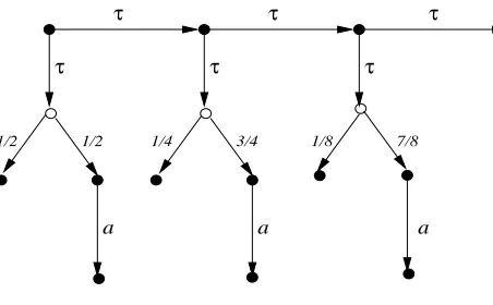
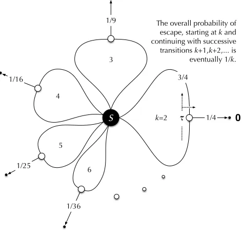
Example 3.16 Consider the (infinite) collection of statesskand probabilitiespkfork≥2such that

sk −→τ [a℄

pk⊕sk+1,

where we choosepkso that starting from anyskthe probability of eventually taking a left-hand branch, and so reaching

[a℄ultimately, is just1/kin total. Thuspk must satisfy1/k=pk+ (1−pk)/(k+1), whence by arithmetic we have

thatpk:= 1/k2will do. Therefore in particulars2=⇒ 1₂[a℄, with the remaining

1

(11)

Our final example demonstrates that derivatives of (interpretations of)pCSPprocesses may have infinite support, and hence that we can have[P℄=⇒∆

′_{such that there is no}_P′_∈_pCSP_with

[P

′

℄= ∆

′_.

Example 3.17 LetPdenote the processrecx. b1

2⊕(x|∅0). Then we have the derivation:

[P℄ = [P℄+ε

[P℄

τ

−→ 1

2·[P |∅0

1

℄+

1 2·[b℄

1

2·[P|∅0

1

℄

τ

−→ 1

22·[P |∅0

2

℄+

1

22·[b|∅0

1

℄

. . . . 1

2k·[P |∅0

k

℄

τ

−→ 1

2k+1·[P |∅0

k+1

℄+

1

2k+1·[b|∅0

k

℄

. . .

where0krepresentskinstances of0running in parallel. This implies that

[P℄=⇒Θ

where

Θ =X

k≥1

1

2k·[b|∅ 0

k

℄

a distribution with infinite support. 2

3.3 Properties of weak derivations

Here we develop some properties of the weak move relation=⇒which will be important later on in the paper. We wish to use weak derivation as much as possible in the same way as the lifted action relations−→α , and therefore we start with showing that=⇒enjoys two of the most crucial properties of−→α : linearity of Definition 3.2 and the decomposition property of Proposition 3.9.

Theorem 3.18 Supposep1+p2≤1. Then

(i) ∆1,2=⇒∆′1,2implies(p1·∆1+p2·∆2) =⇒(p1·∆1′ +p2·∆′2).

(ii) If(p1·∆1+p2·∆2) =⇒∆′then∆′=p1·∆′1+p2·∆′2for subdistributions∆′1,2such that∆1,2=⇒∆′1,2.

Proof: For (i) we note that lifted transitions−→τ have that property directly from Clause (2) of Definition 3.2. Thus the structures whose existence is implied by Definition 3.12 for∆1=⇒∆′1and∆2=⇒∆′2separately can be added with

thep1, p2scaling given to form a single composite structure establishing(p1·∆1+p2·∆2) =⇒(p1·∆′1+p2·∆′2).

For (ii) we use an inductive argument. To avoid confusion of subscripts we will effect some renaming and simpli-fication in the demonstrandum, making it read

IfΓ + Λ =⇒ΠthenΠ = ΠΓ+ ΠΛwithΓ,Λ =⇒ΠΓ,Λ_. ₍₂₎

(Thep1,2will be re-introduced further below.)

Now from Definition 3.12 we haveΓ + Λ = Π0= Π×0 + Π→0 for someΠ0×,Π→0 with, further, thatΠ→0 −→τ Π1

for someΠ1. For anys∈S, define

Γ→_{(s) :=} _min(Γ(s),_Π→

0 (s))

Γ×_{(s) :=} _Γ(s)₋_Γ→_(s) Λ×_{(s) :=} _min(Λ(s),_Π×

0(s))

Λ→_{(s) :=} _Λ(s)₋_Λ×_(s)_,

(12)

and then check these elementary facts: thatΓ×+ Γ→ = ΓandΛ× + Λ→ = Λ, and that all the introduced sub-distributions are in their proper ranges. What remains is to show that they combine properly, and for that we fix a state sand distinguish two cases: either (a) Π→0 (s) ≥ Γ(s)or (b) Π→0 (s) ≤ Γ(s). In Case (a) the definitions

2 (3) simplify to Γ→(s) = Γ(s),Γ×(s) = 0,Λ×(s) = Π0×(s)andΛ→(s) = Λ(s)−Π×0(s), whence immediately

Γ→(s) + Λ→(s) = Π→0 (s)andΓ×(s) + Λ×(s) = Π×0(s). Case (b) is similar.

BecauseΠ→

0 is−→τ -enabled, we see thats−→τ6 impliesΠ→0 (s) = 0whence alsoΓ→(s) = Λ→(s) = 0, so that

bothΓ→_,_Λ→_are_−→τ _{-enabled also. Thus we appeal to Proposition 3.9 to find}_Γ

1,Λ1withΓ→−→τ Γ1andΛ→−→τ Λ1

andΠ1= Γ1+ Λ1.

Being now in the same position withΠ1as we were withΠ0, we can continue this procedure (here the informal

induction) to induce derivation structures forΓ,Λseparately that establish (2) when added together as in Part (i) of this lemma.

Finally, we letΓ,Λ,Πbep1·∆1, p2·∆2,∆′, and scale the induced derivation structures up by1/p1,1/p2

respec-tively. Because later subdistributions in those structures can never be bigger than earlier ones, the proper bounding of ∆1,2themselves guarantees that the up-scaling does not make any subsequent subdistributions too big. 2

With Theorem 3.18, the relation=⇒ ⊆ D(S)× D(S)can be obtained as the lifting of a relation=⇒SfromSto D(S), which is defined by writings=⇒S Θjust whens=⇒Θ.

Proposition 3.19 (=⇒S) = (=⇒).

Proof: That∆ =⇒S Θimplies∆ =⇒Θis a simple application of Part (i) of Theorem 3.18. For the other direction,

suppose∆ =⇒ Θ: given that∆ =P

s∈⌈∆⌉∆(s)·s, Part (ii) of the same lemma enables us to decomposeΘinto

P

s∈⌈∆⌉∆(s)·Θs wheres =⇒ Θsfor each s in⌈∆⌉. But the latter actually means thats =⇒S Θs, and so by

definition this implies∆ =⇒S Θ. 2

It is immediate that the relations=⇒is convex because of its being a lifting.

We proceed with the important properties of reflexivity and transitivity of weak derivations. First note that reflex-ivity is straightforward; in Definition 3.12 it sufficies to take∆→

0 to be the empty distributionε.

Theorem 3.20 (Transitivity of=⇒) If∆ =⇒ΘandΘ =⇒Λthen∆ =⇒Λ.

Proof: By definition∆ =⇒Θmeans that some∆k,∆k×,∆→k exist for allk≥0such that

∆ = ∆0, ∆k = ∆×_k + ∆→k , ∆→k −→τ ∆k+1, Θ =

∞

X

k=0

∆×_k. (4)

SinceΘ = ∆×0 +

P

k≥1∆×k andΘ =⇒Λ, by Theorem 3.18 there areΛ0,Λ

≥

1 such that

∆×0 =⇒Λ0,

X

k≥1

∆×_k =⇒Λ≥1, Λ = Λ0+ Λ≥1 .

Using Theorem 3.18 again, we haveΛ1,Λ≥2 such that

∆×₁ =⇒Λ1,

X

k≥2

∆×_k =⇒Λ≥₂, Λ≥₁ = Λ1+ Λ≥2,

thus in combinationΛ = Λ0+ Λ1+ Λ≥2. Continuing this process we have that

∆×_k =⇒Λk,

X

j>k

∆×_j =⇒Λ≥_k₊₁, Λ =

k

X

j=0

Λj+ Λ≥_k+1 (5)

(13)

for allk≥0. Lemma 3.5 and Proposition 3.19 ensure that∆ =⇒Θimplies|∆| ≥ |Θ|for any subdistributions∆and Θ, and therefore that|P

j>k∆×j| ≥ |Λ

≥

k+1|for allk≥0. But sinceΘ =

P∞

k=0∆×k from (4), we know that the tail

sumP

j>k∆

×

j converges toεwhenkapproaches∞, and therefore thatlimk→∞Λ≥k =ε. Thus by taking that limit

we conclude that

Λ =

∞

X

k=0

Λk. (6)

Now for eachk≥0, we know that∆×_k =⇒Λkgives us some∆kl,∆×kl,∆→kl forl≥0such that

∆×_k = ∆k0, ∆kl = ∆×_kl+ ∆→kl, ∆→kl −→τ ∆k,l+1 Λk=

X

l≥0

∆×_kl. (7)

Therefore we can put all this together with

Λ =

∞

X

k=0

Λk =

X

k,l≥0

∆×_kl = X

i≥0



 X

k,l|k+l=i

∆×_kl



 , (8)

where the last step is a straightforward diagonalisation.

Now from the decompositions above we re-compose an alternative trajectory of∆′i’s to take∆ via =⇒to Λ

directly. Define

∆′i= ∆′×i + ∆′→i , ∆′×i =

X

k,l|k+l=i

∆×_kl, ∆′→i = (

X

k,l|k+l=i

∆→kl) + ∆→i , (9)

so that from (8) we have immediately that

Λ = X

i≥0

∆′×i . (10)

We now show that

(i) ∆ = ∆′

0

(ii) ∆′→

i −→τ ∆′i+1

from which, with (10), we will have∆ =⇒Λas required. For (i) we observe that

∆

= ∆0 (4)

= ∆×0 + ∆→0 (4)

= ∆00+ ∆→0 (7)

= ∆×00+ ∆→00+ ∆→0 (7)

= (P

k,l|k+l=0∆×kl) + (

P

k,l|k+l=0∆→kl) + ∆→0 index arithmetic

= ∆′×

0 + ∆′→0 (9)

= ∆′

0. (9)

For (ii) we observe that

∆′→

i

= (P

k,l|k+l=i∆→kl) + ∆→i (9)

τ

−→ (P

k,l|k+l=i∆k,l+1) + ∆i+1 (4), (7), Proposition 3.9

= (P

k,l|k+l=i(∆×k,l+1+ ∆→k,l+1)) + ∆×i+1+ ∆→i+1 (4), (7)

= (P

k,l|k+l=i∆×k,l+1) + ∆×i+1+ (

P

k,l|k+l=i∆→k,l+1) + ∆→i+1 rearrange

= (P

k,l|k+l=i∆×k,l+1) + ∆i+1,0+ (Pk,l|k+l=i∆→k,l+1) + ∆→i+1 (7)

= (P

k,l|k+l=i∆×k,l+1) + ∆×i+1,0+ ∆→i+1,0+ (

P

(14)

= (P

k,l|k+l=i+1∆×kl) + (

P

k,l|k+l=i+1∆→kl) + ∆→i+1 index arithmetic

= ∆′×

i+1+ ∆′→i+1 (9)

= ∆′

i+1, (9)

which concludes the proof.

2

Finally, we need a property that is the converse of transitivity: if one executes a given weak derivation partly, by stopping more often and moving on less often, one makes another weak transition that can be regarded as an initial segment of the given one. We need the property that after executing such an initial segment, it is still possible to complete the given derivation.

Definition 3.21 A weak derivationΦ =⇒Γis called an initial segment of a weak derivationΦ =⇒Ψif fork ≥0 there areΓk,Γ→k ,Γ×k,Ψk,Ψ→k ,Ψ×k ∈ D(S)such thatΓ0= Ψ0= Φand

Γk = Γ→k + Γ×k Ψk= Ψ→k + Ψ×k Γ→k ≤Ψ→k

Γ→_k −→τ Γk+1 Ψ_k→−→τ Ψk+1 Γk≤Ψk

Γ =P∞

i=0Γ×k Ψ =

P∞

i=0Ψ×k (Ψ→k −Γ→k ) τ

−→(Ψk+1−Γk+1).

Intuitively, in the derivationΦ =⇒ Ψ, for eachk ≥ 0, we only allow a portion ofΨ→_k to makeτ moves, and the rest remains unmoved even if it can enableτ moves, so as to obtain an initial segmentΦ =⇒ Γ. Accordingly, each Γ×_k includes the corresponding unmoved part ofΨ→k , which is eventually collected inΓ. Now fromΓif we let those

previously unmoved parts perform exactly the sameτmoves as inΦ =⇒Ψ, we will end up with a derivation leading toΨ. This is formulated in Proposition 3.22; the proof is tedious thus omitted.

Proposition 3.22 IfΦ =⇒Γis an initial segment ofΦ =⇒Ψ, thenΓ =⇒Ψ. 2

4 Testing probabilistic processes

This section is divided into three. Applying a test to a process results in a nondeterministic, but possibly probabilistic, computation structure. The main conceptual issue is how to associate outcomes with these nondeterministic structures. In the first subsection we outline a general approach in which intuitively the nondeterministic choices are resolved implicitly in a dynamic manner. In the second section we describe an alternative approach in which we explicitly associate with a nondeterministic structure a set of deterministic computations, each of which determines a possible outcome. In the final section we show that although these approaches are formally quite different they lead to exactly the same testing preorders.

4.1 Applying a test to a process

We now retrace our earlier approach [3, 2] to the testing of probabilistic processes. A test is simply a process in the languagepCSP, except that it may in addition use special success actions for reporting outcomes: these are drawn from a setΩof fresh actions not already inActτ. We refer to the augmented language aspCSPΩ, and the pLTS it

generates aspltst. Formally a testT is some process from that language, and to apply testTto processPwe form the processT |Act P in which all visible actions ofP must synchronise withT. The resulting composition is a process whose only possible actions areτ and the elements ofΩ. We will define the resultA(T, P)of applying the testT to the processP to be a set of testing outcomes, exactly one of which results from each resolution of the choices in T |Act P. Each testing outcome is anΩ-tuple of real numbers in the interval [0,1], i.e. a functiono: Ω→[0,1], and itsω-componento(ω), forω∈ Ω, gives the probability that the resolution in question will reach anω-success state, one in which the success actionωis possible.

(15)

and vector-based testing in [23]. As in [2], our prime interest here is in scalar testing, but we use vector-based testing as an indispensable tool for establishing our results. To this end we employ a result from [4] saying that for finite-state probabilistic processes, scalar and vector-based testing give rise to the very same testing preorders.

3 Secondly, following [4, 2] we distinguish between state-based and action-based testing. The former is what we described above: success actions are merely used as a method to define success states; a method that bypasses the need to formally introduce state predicates in the operational semantics of our language. In action-based testing, on the other hand, it is the actual execution of a success action that constitutes success, ando(ω)gives the probability that the resolution in question will perform the actionω. State-based testing is employed in [5, 7, 24, 3], and action-based testing in [23, 4]. In [2] it has been shown that for finite probabilistic processes (obtained by dropping the recursion construct frompCSP) the state-based and based testing preorders coincide. This allowed us to use action-based testing to obtain results about state-action-based testing. However, [2] also provides an example showing that for the language considered in the present paper, the two approaches are different, in particular that state-based must testing is more discriminating than action-based must testing. The same example also applies to the non-probabilistic world and, for finitely branching processes, it is the state-based must-testing preorder that coincides with the CSP refinement preorder based on failures and divergences [1, 9, 20]. It is in part for this reason that we employ state-based testing in the current paper.

Whereas state-based scalar testing as well as action-based scalar-and vector-based testing have been used pre-viously in the literature, our use of state-based vector-based testing is new. Since we use this concept merely as a method for proving results about state-based scalar testing, we are not concerned about the generality of our tests for conceptual reasons; any notion of state-based vector-based testing that works in our proofs would be acceptable, as long as the special case of state-based scalar testing agrees with the definitions found in the literature. Here we restrict attention to tests in which no state is simultaneously anω-success state for different values ofω. In fact, we can go further by ruling out all tests in which from one success state one can reach another one, with a different success value.

Definition 4.1 An Ω-test is a closed pCSPexpressionT, but allowing the enriched alphabetActτ ∪Ωof actions

instead of justActτ, such that ift−→ω1 andu−→ω2 forω1, ω2∈Ωwithtreachable fromT andufromt, thenω1=ω2.

Note that for the special case of scalar state-based testing the above restriction is void. In [4], working in an action-based framework, following [23], we didn’t put such a restriction in our definition of testing, but showed, in Ap-pendix A: “One Success Never Leads to Another” that imposing it does not change the resulting testing preorders. Also note that the compositionT |Act P of anΩ-testT and apCSPprocessP is again anΩ-test (i.e. satisfying the requirement of Definition 4.1).

Intuitively, the application of a testT to a processP has an outcomeo ∈ [0,1]Ω_{if we can imagine an army —}

with a continuum of soldiers — marching through our pLTS, starting from the distribution[T |Act P℄, of which, for

ω ∈ Ω, a fractiono(ω) ∈ [0,1]eventually reaches anω-success state. Each time a fragment of the army ends up in a non-success state, it splits up in arbitrary proportions among the outgoing transitions of that state (which are all labelledτ). If such a transition ends up in a distribution∆then, fors∈ ⌈∆⌉, a fraction∆(s)of the fragment that took that transition ends up in states. The army begins its march by being distributed over the initial distribution[T |Act P℄

in the same vein. As soon as a fragment of the army reaches anω-success state, it stops marching, and the size of that fragent is counted towardso(ω). Definition 4.1 ensures that in such a case there is no ambiguity about which success action the division contributes to. Definition 4.1 also ensures that there is no point in marching any further. The total success valueP

ω∈Ωo(ω)must be in the interval [0,1]; it represents the fraction of the army eventually reaching a

success state of any kind. The unsuccessful part of the army1−P

ω∈Ωo(ω)represents the fraction that either got

stuck in a deadlock state, one without outgoing transitions, or that will march forever. In general we get different outcomeso∈ A(T, P)for each possible way a fragment in a non-success and non-deadlock state can partition itself among the outgoing transitions of that state.

We will now formalise this intuition by a definition ofA(T, P). Our definition has three ingredients. First of all we normalise our pLTS by removing allτ-transitions that leave a success state. This way anω-success state will only have outgoing transitions labelledω. This prevents our army from scooting past a success state.

Definition 4.2 [ω-respecting]. LethS, L,→ibe a pLTS such that the set of labels LincludesΩ. It is said to be ω-respecting whenevers_−→ω _{, for any}_ω_∈_Ω_,_s_−→τ₆ _.

(16)

It is straightforward to modify an arbitrary pLTS so that it isω-respecting. Here we outline how this is done for our pLTS forpCSP.

Definition 4.3 [Pruning] Let[·]be the unary operator onΩ-test states given by the operational rules

s−→ω ∆

[s]_−→ω _[∆] (ω∈Ω)

s−→ω6 (for allω∈Ω), s−→α ∆

[s]_−→α _[∆] (α∈Actτ).

Just as2and|A, this operator extends as syntactic sugar toΩ-tests by distributing[·]overp⊕; likewise, it extends to distributions by[∆]([s]) = ∆(s). Clearly, this operator does nothing else than removing all outgoing transitions of a success state other than the ones labelled withω ∈Ω. Applying this operator, we can just as well envision our army to have started marching from the distribution[[T |Act P]℄; it will continue marching alongτ-transitions for as long

asτ-transitions are possible, and will halt in statesiffs_−→τ6 _{, which is the case iff}_s_{is either a success or a deadlock}

state.

Next, using Definition 3.12, we characterise the set of subdistributions Θthat can be reached by an army as envisioned above at the end of its march from[[T |Act P]℄. In generalΘneed not be a total distribution: the mass

|Θ|represents the fraction of the army that eventually stops marching and thus reachesΘ. The remaining fraction 1− |Θ|of the army marches on forever. A march of an army as described above can be modelled perfectly by a weak transition[[T |Act P]℄=⇒Θas defined in Section 3.2. The end subdistributionΘof this march has the property that

there is no nontrivial weak transitionΘ =⇒. System states with this property are traditionally called stable.

Definition 4.4 [Extreme derivatives] A statesin a pLTS is called stable ifs_−→τ6 _{, and a subdistribution}_Θ_{is called}

stable if every state in its support is stable. We write∆ =⇒≻Θwhenever∆ =⇒ΘandΘis stable, and callΘan extreme derivative of∆.

Referring to Definition 3.12, we see this means that in the extreme derivation ofΘfrom∆at every stage a state must move on if it can, so that every stopping component can contain only states which must stop: fors∈∆→

k + ∆×k we

haves ∈ ∆×_k if and now also only ifs_−→τ6 _{. Moreover if the pLTS is}_ω_{-respecting then whenever}_s _∈_∆→

k , that is

whenever it marches on, it is not successful,s_−→ω6 _{for every}_ω_∈_Ω_.

Lemma 4.5 [Existence of extreme derivatives]

(i) For every subdistribution∆there exists some (stable)∆′ _{such that}_{∆ =}_⇒≻_∆′_.

(ii) In a deterministic pLTS we have that∆ =⇒≻∆′and∆ =⇒≻∆′′implies∆′= ∆′′.

Proof: We construct a derivation as in Definition 3.12 of a stable∆′ _{by defining the components}_∆

k,∆×k and∆→k

using induction onk. Let us assume that the subdistribution∆k has been defined; in the base casek = 0this is

simply∆. The decomposition of this∆kinto the components∆×k and∆→k is carried out by defining the former to be

precisely those states which must stop, i.e. thosesfor whichs−→τ6 . Formally∆×_k is determined by:

∆×_k(s) =

(

∆k(s) if s−→τ6

0 otherwise

Then∆→

k is given by the remainder of∆k, namely those states which can perform aτaction:

∆→k (s) =

(

∆k(s) if s−→τ

0 otherwise

Note that these definitions divide the support of∆k into two disjoints sets, namely the support of∆×k and the support

of∆→

k . Moreover by construction we know that∆→k τ

−→Θfor someΘ; we let∆k+1be an arbitrary suchΘ.

This completes our definition of an extreme derivative as in Definition 3.12 and so we have established (i). For (ii) we observe that in a deterministic pLTS the above choice of∆k+1is unique, so that the whole derivative

(17)

It is worth pointing out that the use of subdistributions, rather than distributions, is essential here. If∆diverges, that is if there is an infinite sequence of derivations∆−→τ ∆1−→τ . . .∆k −→τ . . ., then the only extreme derivative of∆is

the empty subdistributionε. For example the only transition ofrecx. xisrecx. x−→τ recx. x, and thereforerecx. x diverges; consequently its unique extreme derivative isε.

The final ingredient in the definition of the set of outcomesA(T, P)is to use this notion of extreme derivative to formalise the subdistributions that can be reached from[[T |Act P]℄at the end of the march of an army as envisioned

above; each extreme derivativeΘmodels the end of a march of our army. All statess∈ ⌈Θ⌉either satisfys_−→ω _for

an uniqueω∈Ω, or haves6→.

Definition 4.6 [Outcomes] The outcome$Θ∈[0,1]Ω_{of a stable subdistribution}_Θ_{is given by}_{$Θ(ω) =} X

s∈⌈Θ⌉, s−→ω

Θ(s).

Putting all three ingredients together, we arrive at a definition ofA(T, P):

Definition 4.7 LetPbe apCSPprocess andTanΩ-test. ThenA(T, P) ={$Θ|[[T |ActP℄] =⇒≻Θ}.

The role of pruning in the above definition can be seen via the following example.

Example 4.8 LetP =a.b.0andT =a.(b.02_ω.₀₎_{. The pLTS generated by applying}_T _to_P_{can be described by} the processτ.(τ.02_ω.₀₎. Then[T |ActP℄has a unique extreme derivation[T |ActP℄=⇒≻[0℄, and[[T |Act P℄]

also has a unique extreme derivation[[T |ActP℄] =⇒≻[ω.0℄. The outcome inA(T, P)shows that processP passes

testTwith probability1, which is what we expect for state-based testing, which we use in this paper. Without pruning we would get an outcome saying thatPpassesTwith probability0, which would be what is expected for action-based

testing. 2

There are two standard methods for comparing two sets of outcomes:

O1≤HoO2 if for everyo1∈O1there exists someo2∈O2such thato1≤o2

O1≤Sm O2 if for everyo2∈O2there exists someo1∈O1such thato1≤o2

This gives us our definition of the may- and must-testing preorders; they are decorated with·Ω_{for the repertoire}_Ω_of

testing actions they employ.

Definition 4.9

1. P ⊑Ω

pmayQif for everyΩ-testT,A(T, P)≤HoA(T, Q).

2. P ⊑Ω

pmustQif for everyΩ-testT,A(T, P)≤Sm A(T, Q).

These preorders are abbreviated toP ⊑pmay Q, andP ⊑pmustQ, when|Ω|= 1.

Here are two examples of these preorders.

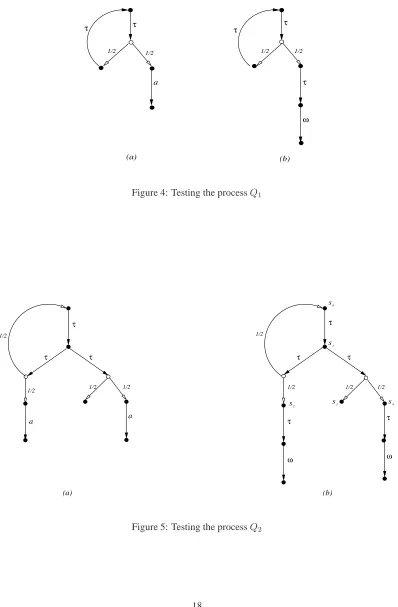
Example 4.10 Consider the processQ1 =recx.(τ.x1

2⊕a), which was already discussed in the Introduction, Fig-ure 1(a). When we apply the testT = a.ω to it we get the pLTS in Figure 4(b), which is deterministic, hence unaffected by pruning; from part (ii) of Lemma 4.5 it follows thats0has a unique extreme derivativeΘ. MoreoverΘ

can be calculated to be

X

k≥1

1 2k ·ω,

which simplifies to the distributionω. Thus is the same set of results gained by applyingTtoaon its own; and in fact it is possible to show that this holds for all tests, giving

Q1≃pmaya Q1≃pmusta .

(18)

τ

1/2 1/2

τ

1/2 1/2

τ τ

a

ω τ

[image:18.612.109.507.61.668.2]

(b) (a)

Figure 4: Testing the processQ1

1/2 1/2

τ

a

τ τ τ

1/2 1/2

τ

ω

(a) (b)

τ τ

1/2 1/2

s0

s1

s3 s4

a

1/2

ω τ

1/2

[image:18.612.192.418.67.231.2]

s2

(19)

4 Example 4.11 Consider the processQ2 = recx. τ.(x 1

2⊕ a) 2 τ.(0 12⊕ a)and the application of the same test T =a.ωto it, as outlined in Figure 5(a) and (b).

Consider any extreme derivative∆′ from[[T |Act Q2℄], which we have abbreviated tos0; note that here again

pruning actually has no effect. Using the notation of Definition 3.12, it is clear that∆×0 and∆→0 must beεands0

respectively. Similarly,∆×₁ and∆→

1 must beεands1respectively. Buts1 is a nondeterministic state, having two

possible transitions:

(i) s1−→τ Θ0whereΘ0has support{s0, s2}and assigns each of them the weight1₂

(ii) s1−→τ Θ1whereΘ1has the support{s3, s4}, again diving the mass equally among them.

So there are many possibilities for∆1; Lemma 3.4 shows that in fact∆2can be of the form

p·Θ0+ (1−p)·Θ1 (11)

for any choice ofp∈[0,1].

Let us consider one possibility, an extreme one wherepis chosen to be0; only the transition (ii) above is used. Here∆→2 is the subdistribution 12s4, and∆→k =εwheneverk >2. A simple calculation shows that in this case the

extreme derivative generated isΘe

1=12ωwhich implies that 1

2 ∈ A(T, Q2).

Another possibility for∆2 isΘ0, corresponding to the choice of p = 1in (11) above. Continuing with this

derivation leads to∆3being 1₂·s1+1₂·ω; in other words∆×3 =12·ωand∆→3 =12·s1. Now in the generation of∆4

from∆→

3 once more we have to resolve a transition from the nondeterministic states1, by choosing some arbitrary

p∈[0,1]in (11). Suppose that each time this arises we systematically choosep= 1, that is, we ignore completely the transition (ii) above. Then it is easy to see that the extreme derivative generated is

Θe0=

X

k≥1

1 2k ·ω

which simplifies to the distributionω. This in turn means that1∈ A(T, Q2).

We have seen two possible derivations of extreme derivatives from s0. But there are many others. In general

whenever∆→k is of the formq·s1 we have to resolve the nondeterminism by choosing ap ∈ [0,1]in (11) above;

moreover each such choice is independent. However it will follow from later results, specifically Corollary 6.10, that every extreme derivative∆′_of_s

0is of the form

q·Θe

0+ (1−q)Θe1

for some choice ofq∈[0,1]; this is explained in Example 6.11. Consequently it follows thatA(T, Q2) = [1₂,1].

SinceA(T, a) ={1}it follows that

A(T, a) ≤Ho A(T, Q2) A(T, Q2) ≤Sm A(T, a).

Again it is possible to show that these inequalities result from any testTand that therefore we have

a⊑pmay Q2 Q2⊑pmusta

2

4_{The process and diagram do not match exactly, as unwinding the recursion takes a}_τ_{-step. Also I need the states enumerated}_s

0, . . . s4both here and in Example 6.11.

(20)

4.2 Using explicit resolutions

The derivation of extreme derivations, via the schema in Definition 3.12, involves the systematic dynamic resolution of nondeterministic states, in each transition from ∆→_k to∆k+1. In the literature various mechanisms have been

proposed for making these choices; for example policies are used in [21], adversaries in [14], schedulers in [22], . . . . Here we concentrate not on any such mechanism but rather the results of their application. In general they reduce a nondeterministic structure, typically a pLTS, to a set of deterministic structures. To describe these determinstic structures we adapt the notion of resolution defined in [23, 4] for probabilistic automata, to pLTSs.

Definition 4.12 [Resolutions] A resolution of a subdistribution∆∈ D(S)in a pLTShS,Ωτ,→iis a triplehR,Θ,→Ri

wherehR,Ωτ,→Riis a deterministic pLTS andΘ∈ D(R), such that there exists a resolving functionf ∈ R → S

satisfying

(i) Img_f(Θ) = ∆

(ii) ifr−→α RΘ′forα∈Ωτthenf(r)−→α Imgf(Θ′)

(iii) iff(r)_−→α _for_α_∈_Ω

τthenr−→α R.

The reader is referred to Section 2 of [4] for a detailed discussion of this concept of resolutions, and the manner in which it represents computation runs of a process; in particular in a resolution states inSare allowed to be resolved into distributions, and computation steps can be probabilistically interpolated.

We now explain how to associate an outcome with a particular resolution, which in turn will associate a set of outcomes with a subdistribution in a pLTS. Given a deterministic pLTShR,Ωτ,→iconsider the functionalR: (R→

[0,1]Ω₎_→_(R_→_[0,_1]Ω₎_{defined by}

R(f)(r)(ω) :=



 

 

1 ifr−→ω

0 ifr_−→ω6 _and_r_−→τ₆

Exp_∆(f)(ω) ifr−→ω6 andr−→τ ∆.

(12)

We view the unit interval[0,1]ordered in the standard manner as a complete lattice; this induces the structure of a

5

complete lattice on the product[0,1]Ω_{and in turn on the set of functions}_R_→_[0,_1]Ω_{. The functional}_R_{is easily seen}

to be monotonic and therefore has a least fixpoint, which we denote byV_h_R,_Ω

τ,→i; this is abbreviated toVwhen the resolution in question is understood.

Now letAr_{(T, P}₎_{denote the set of vectors}

{Exp_Θ(V_h_R,_Ω

τ,→i) | hR,Θ,→iis a resolution of[T |ActP℄}.

Note that here we use resolutions of[T |Act P℄rather than its pruning[[T |Act P℄]. This is because the functionalR,

and therefore its least fixpointV, has pruning built-in; that isRis defined so thatV_{(s) =}V_([s]).

Definition 4.13 Given twopCSPprocessesPandQ,

• P ⊑Ω

rpmayQif for everyΩ-testT, we haveAr(T, P)≤HoAr(T, Q)

• P ⊑Ω

rpmustQif for everyΩ-testT, we haveAr(T, P)≤SmAr(T, Q).

Example 4.14 (revisiting Example 4.10) The pLTS in Figure 4(b) is already deterministic, hence has only one

reso-lution, itself. Moreover the outcomeVassociated with it is determined by its value at the states0. This in turn is the

least solution of the equation

V_(s₀_{) =}1

2 ·V(s0) + 1 2 In fact this equation has a unique solution in[0,1], namely1. ThusAr_{(T, Q}

1) ={1}. 2

5_{I have taken this definition of}_R_{from Concur; it can be simplified if the pLTS is assumed to be}_ω_{-respecting. It is different than}_R_{used in}

(21)

Example 4.15 (revisiting Example 4.11) Here we reuse the notation of Example 4.11.

Consider the processQ2=recx. τ.(τ.x1

2⊕a)2τ.(012⊕a)and the application of the testT =a.ωto it; this is outlined in Figure 5. In the pLTS ofT |Act Q2, for eachk≥1there is a resolutionRk such thatV(Rk) = (1−₂1k); intuitively it goes around the loop(k−1)times before at last taking the right handτaction. ThusAr_{(T, Q}

2)contains

(1− 1

2k)for everyk ≥ 1. But it also contains1, because of the resolution which takes the left handτ-move every time. ThusAr_{(T, Q}

2)includes the set

{(1−1

2), (1− 1

22), . . . ,(1−

1

2k), . . . 1}

From later results it will follow thatAr_{(T, Q}

2)is actually the convex closure of this set, namely[1₂,1].

Also look at ability ofQ2to refusea. 2

4.3 Comparison

We have now seen two ways of associating sets of outcomes with the application of a test to the process. The first, in Section 4.1, uses extreme derivations in which nondeterministic choices are resolved dynamically as the derivation proceeds, while in the second, in Section 4.2, we associate with a test and a process a set of deterministic structures called resolutions. In this section we show that the testing preorders obtained from these two aproaches coincide.

First let us see how an extreme derivation can be viewed as a method for dynamically generating a resolution.

Theorem 4.16 (Resolutions from extreme derivatives) Suppose∆ =⇒≻∆′ _{in a pLTS}_h_S,_Ω

τ,→i. Then there is a

resolutionhR,Θ,→Riof∆, with resolving functionf, such thatΘ =⇒≻RΘ′for someΘ′such that∆′=Imgf(Θ′).

Proof: Consider an extreme derivation of∆ =⇒≻ ∆′, as given in Definition 3.12 where all∆×_k are assumed to be stable. To define the corresponding resolutionhR,Θ,−→Riwe refer to Definition 4.12. First let the set of statesRbe

S×Nand the resolving functionf:R→Sbe given byf(s, k) =s. To complete the description we must define the partial functions−→α , forα=ωandα=τ. These are always defined so that if(s, k)_−→α _Γ_{then the only states in}

the support ofΓare of the form(s′_{, k}_{+ 1)}_{. In the definition we use}_Θ↓k_{, for any subdistribution}_Θ_over_S_{, to be the}

subdistribution overRgiven by

Θ↓k(t) =

(

Θ(s) ift= (s, k)

0 otherwise

Note that by definition

(a) Img_f(Θ↓k_{) = Θ}

(b) ∆↓_kk = ∆→↓_k k+ ∆×↓_k k

The definition of−→ω R is straightforward: its domain consists of states(s, k)wheres∈ ⌈∆×_k⌉and is defined by

letting(s, k)_−→ω _∆↓k+1

s for some arbitrarily chosens−→ω ∆s.

The definition of−→τ Ris more complicated, and is determined by the moves∆→k −→τ ∆k+1. For a givenkthis

move means that

∆→k =

X

i∈I

pi·si, ∆k+1=

X

i∈I

pi·Γi, si−→τ Γi

So for eachkwe let

(s, k)−→τ R

X

si=s

pi·Γ↓_ik+1

Testing Finitary Probabilistic Processes