A system for learning statistical motion patterns

BIROn - Birkbeck Institutional Research Online

Hu, W. and Xiao, X. and Fu, Z. and Xie, D. and Tan, T. and Maybank, Stephen

J. (2006) A system for learning statistical motion patterns. IEEE Transactions

on Pattern Analysis and Machine Intelligence 28 (9), 1450 -1464.. ISSN

0162-8828.

Downloaded from:

Usage Guidelines:

Please refer to usage guidelines at

or alternatively

Birkbeck ePrints: an open access repository of the

research output of Birkbeck College

http://eprints.bbk.ac.uk

Hu, Weiming; Xiao, Xuejuan; Fu, Zhouyu; Xie, Dan; Tan,

Tieniu and Maybank, Steve (2006). A system for learning statistical

motion patterns. IEEE Transactions on Pattern Analysis and

Machine Intelligence 28 (9)1450 –1464.

This is an exact copy of a paper published in

IEEE Transactions on Pattern

Analysis and Machine Intelligence

(ISSN 0162-8828). It is reproduced with

permission from the publisher. Personal use of this material is permitted.

However, permission to reprint/republish this material for advertising or

promotional purposes or for creating new collective works for resale or

redistribution to servers or lists, or to reuse any copyrighted component of this

work in other works must be obtained from the IEEE. © 2006 IEEE.

Copyright and all rights therein are retained by authors or by other copyright

holders. All persons downloading this information are expected to adhere to

the terms and constraints invoked by copyright. This document or any part

thereof may not be reposted without the explicit permission of the copyright

holder.

Citation for this copy:

Hu, Weiming; Xiao, Xuejuan; Fu, Zhouyu; Xie, Dan; Tan, Tieniu and

Maybank, Steve (2006). A system for learning statistical motion patterns.

London: Birkbeck ePrints.

Available at:

http://eprints.bbk.ac.uk/archive/00000442

Citation as published:

Hu, Weiming; Xiao, Xuejuan; Fu, Zhouyu; Xie, Dan; Tan, Tieniu and

Maybank, Steve (2006). A system for learning statistical motion patterns.

IEEE Transactions on Pattern Analysis and Machine Intelligence 28

(9)1450 –

1464.

http://eprints.bbk.ac.uk

A System for Learning

Statistical Motion Patterns

Weiming Hu, Xuejuan Xiao, Zhouyu Fu, Dan Xie, Tieniu Tan,

Fellow

,

IEEE

, and

Steve Maybank,

Member

,

IEEE

Abstract—Analysis of motion patterns is an effective approach for anomaly detection and behavior prediction. Current approaches for the analysis of motion patterns depend on known scenes, where objects move in predefined ways. It is highly desirable to automatically construct object motion patterns which reflect the knowledge of the scene. In this paper, we present a system for automatically learning motion patterns for anomaly detection and behavior prediction based on a proposed algorithm for robustly tracking multiple objects. In the tracking algorithm, foreground pixels are clustered using a fast accurate fuzzyK-meansalgorithm. Growing and prediction of the cluster centroids of foreground pixels ensure that each cluster centroid is associated with a moving object in the scene. In the algorithm for learning motion patterns, trajectories are clustered hierarchically using spatial and temporal information and then each motion pattern is represented with a chain of Gaussian distributions. Based on the learned statistical motion patterns, statistical methods are used to detect anomalies and predict behaviors. Our system is tested using image sequences acquired, respectively, from a crowded real traffic scene and a model traffic scene. Experimental results show the robustness of the tracking algorithm, the efficiency of the algorithm for learning motion patterns, and the encouraging performance of algorithms for anomaly detection and behavior prediction.

Index Terms—Tracking multiple objects, learning statistical motion patterns, anomaly detection, behavior understanding.

Ç

1

I

I

computer vision research. One of the most important goals of visual surveillance systems is to track objects and further analyze their behaviors in order to detect anomalies, predict future behaviors, or predict potential abnormal behaviors before they occur. Analysis of motion patterns is an effective approach for anomaly detection and behavior prediction. For the most part, objects in the scene do not move randomly. Instead, they usually follow specific motion patterns. Knowledge of motion patterns can be used to detect anomalous object motions and predict behaviors. Current tracking systems mainly base their analysis of motion patterns on a predefined classification of tracked data. For instance, Collins et al. [8] allocate detected objects to semantic categories such as human, human group, and vehicle. Further classification of human behaviors, such as walking and running, has been achieved. Davis et al. [10] model and recognize a set of behaviors: walking, marching, line-walking, and kicking while walk-ing. However, in most applications, motion patterns of objects cannot be easily predefined. A more appropriate method is to automatically construct object motion patterns which reflect the inherent properties of the scene, without the assumption of any prior knowledge.

Although the automatic construction of motion patterns is a newly emergent research topic, some pioneering investiga-tions of this problem have already been made. Johnson and Hogg [20] learn probability density functions of object trajectories generated from image sequences. The movement of an object is described in terms of a sequence of flow vectors, where each vector consists of four elements representing the position and velocity of the object in the image plane. The patterns of object trajectories are formed with two competi-tive learning networks which are connected by leaky neurons. Both of the neural networks are learned using vector quantization. Johnson [19] describes the enhancement of the model developed in [20] to include generative capabilities via the superimposition of learned prediction schemes. In Johnson’s work, the number of different behaviors is not estimated and the detection probability theory is not used to identify anomalies and predict motions. Stauffer and Grimson [42] learn motion patterns using real-time tracking. Their method involves developing a codebook of representations using an online vector quantization on the entire set of representations acquired by the tracker. Joint cooccurrence statistics are accumulated over the codebook by treating the set of representations in each sequence as an equivalency multiset. Finally, a hierarchical classification is performed using only the accumulated cooccurrence data. In Stauffer and Grimson’ work, the linking relationship between successive positions in a trajectory is not represented in the joint cooccurrence statistics. It is unclear how to detect anomalies using motion patterns. Motion prediction is not involved. Sumpter and Bulpitt [43] present a novel approach for learning long-term spatial-temporal patterns of object motions in image sequences using a neural network para-digm to predict future behaviors. As in [20], they use two neural networks. The first network and the input vector components to the second network are the same as in [20]. They introduce feedback to the second network giving an effective prediction of object behaviors. However, the

. W. Hu, X. Xiao, Z. Fu, D. Xie and T. Tan are with the National Laboratory of Pattern Recognition, Institute of Automation, Chinese Academy of Sciences, PO Box 2728, Beijing 100080, P.R. China.

E-mail: {wmhu, xjxiao, zyfu, dxie, tnt}@nlpr.ia.ac.cn.

. S. Maybank is with the School of Computer Science and Information Systems, Birkbeck College, Malet Street, Bloomsbury, London WC1E 7HX, UK. E-mail: [email protected].

Manuscript received 22 Nov. 2004; revised 9 Oct. 2005; accepted 2 Feb. 2006; published online 13 July 2006.

Recommended for acceptance by I.A. Essa.

For information on obtaining reprints of this article, please send e-mail to: [email protected], and reference IEEECS Log Number TPAMI-0622-1104.

number of input vector components and the number of output neurons in the second network remain equal to the number of flow vectors, so the learning efficiency inevitably decreases when the size of the network increases. Further-more, this neural network structure cannot be used to detect abnormal behaviors. Owens and Hunter [35] determine whether a point on a trajectory is normal using the distributions of flow vectors. Their method does not represent patterns of trajectories, so it can neither recognize behaviors represented by trajectories nor predict them. Bennewitz et al. [2] propose a method for learning motion patterns of people. Data recorded with laser range finders are clustered. Based on the clustering result, a Hidden Markov Model is derived. This Hidden Markov Model is used to predict positions of people from the learned motion patterns. In the method, a linear interpolation is used to ensure that the input trajectories, which are directly used to learn motion patterns, have the same number of positions. This interpola-tion approximates to the sampling of trajectories at a uniform distance interval. The sequential information is omitted. The assumption in [2] that the Gaussian distributions for different positions on different patterns all have a fixed standard deviation does not properly reflect the distribution char-acteristics of motion patterns. Anomaly detection and long-term prediction are not considered. In the experiments, the proposed method is only tested on very small sets of trajectories. Zhong et al. [52] detect anomalies with compar-ison between behaviors but without learned motion patterns. Ellis et al. [12], [25], [26] develop a praiseworthy method for learning entry/exit zones and routes from trajectory samples. The start/end points of trajectories are used to learn entry/ exit zones applying the Expectation-Maximization algo-rithm. For the learning of routes, a new trajectory is compared with all routes already in the database using a simple distance measure. If a match is found, the trajectory is added to the matching route and the route is updated. Otherwise, a new route is initialized. The limitation of the method is that only spatial information is used for trajectory clustering and anomaly detection. Temporal information is not well represented and, thus, behavior prediction is not covered. Junejo et al. [22] apply graph cuts to cluster trajectories using the Hausdorff distance to compare different trajectories and calculate the edge weights of the similarity matrix. The Hausdorff distance compares spatial information only and it does not preserve sequential information. The Hausdorff distance measure does not distinguish between objects following the same route but heading in opposite directions. While “learning motion patterns” and “learning routes (or paths)” [22], [25] are alike, they differ in that even if objects pass along the same route, they may produce different behaviors (motion patterns). For example, a vehicle may rush, move, or worm its way through a route; a person may stroll, walk, or run through a route. These behaviors are treated as different, even if they occur in the same route. Motion patterns contain temporal information which is necessary for the online detection of velocity-related anomalies such as speeding vehicles and traffic incidents and the prediction of future behaviors.

In this paper, we present a system for learning object motion patterns which are then used to detect anomalies and predict behaviors. Our system is original in the following ways:

. Based on clustering foreground pixels using a fast accurate fuzzy K-means algorithm, we propose a

new algorithm for robustly tracking multiple objects. Growing and predictive adaptation are employed to ensure that each cluster centroid is associated with a moving object in the scene. Our algorithm does not need accurate motion segmentation and does not require a complex matching process.

. Based on the fuzzyK-meansalgorithm, we propose a new hierarchical trajectory clustering method. In the method, spatial information is used to cluster all trajectories into some different trajectory categories, each of which is further clustered into subcategories with the temporal information. The number of cluster centroids is estimated. The abnormal trajec-tories in the sample set are processed.

. Based on the clustered trajectories, we learn the characteristics of each motion pattern that is repre-sented by a chain of Gaussian distributions whose standard deviations are derived from the sample trajectories.

. Based on the learned statistical motion patterns, we use statistical theory, together with Bayes rule, to detect anomalies and predict behaviors.

This paper is organized as follows: Section 2 briefly reviews the related work of behavior understanding. Section 3 describes the framework of our system. Section 4 introduces our method for tracking multiple objects. Section 5 presents our algorithm for clustering trajectories and learning statis-tical motion patterns. Section 6 covers our method for anomaly detection and behavior prediction. Section 7 describes experimental results. The last section summarizes the paper.

2

R

W

In the introduction, we reviewed the references which concern construction of motion patterns in order to make clear the motivation for this paper. In this section, the state of the art in behavior understanding [15], [17] is reviewed. The major existing methods for behavior understanding are outlined as follows:

1. Principal Component Analysis (PCA). The PCA, as a statistical approach, has been applied to the recogni-tion of object behaviors. For instance, Yacoob and Black [49] learn behavior models using PCA of a number of exemplar actions.

2. Dynamic Time Warping (DTW). DTW is a template-based dynamic programming matching technique which has been used to match human movement patterns. For instance, Bobick and Wilson [4] use DTW to match an input signal to a deterministic sequence of states.

3. Finite State Machine (FSM). The most important feature of an FSM is its state-transition function. Wilson et al. [47] analyze the explicit structure of natural gestures where the structure is described by an equivalent of a finite state machine.

distribution, observed behaviors can be organized into meaningful states within an HMM. Oliver et al. [34] propose and compare two different state-based learning architectures, namely, HMMs and CHMMs (Coupled Hidden Markov Models) for modeling peoples’ behaviors and interactions. Nguyen et al. [32] present an Abstract Hidden Markov Memory Mode-based approach for recognizing high-level human behaviors. Duong et al. [11] apply the Switch-ing Hidden Semi-Markov Model to learn and recog-nize human behaviors and detect anomalies.

5. Variable Length Markov Models (VLMMs). Unlike HMMs, VLMMs can capture behavioral dependen-cies that may have a variable or long time scale. Galata et al. [14] propose a method for automatically acquiring stochastic models of a behavior. VLMMs are used for the efficient representation of behaviors. 6. Time Delay Neural Network (TDNN). In TDNN, delay units are added to a general static network, and some of the preceding values in a time-varying sequence are used to predict the next value. TDNN has been successfully applied to hand gesture recognition [50] and lip-reading [29].

7. Grammar Techniques (GT). Based on low level features detected by standard independent probabil-istic temporal behavior detectors, a grammar provides longer-range temporal constraints and disambiguates uncertain low-level detections, etc. Brand [5] uses a simple nonprobabilistic grammar to recognize se-quences of discrete behaviors. Ivanov and Bobick [18] describe a probabilistic grammar approach for the detection and recognition of temporally extended behaviors and interactions between multiple objects. Minnen et al. [30] present a system that uses human-specified grammars to recognize a person performing the Towers of Hanoi task from a video sequence by analyzing object interaction behaviors.

8. Bayesian Networks (BNs). BNs offer many advan-tages for using prior knowledge and modeling the dynamic dependencies between parameters of object states. Town [44] uses an ontology to train the structure and parameters of Bayesian networks for behavior recognition. Park and Aggarwal [37] de-scribe a framework for recognizing human actions and interactions. In the framework, the poses of individual body parts are recognized using individual Bayesian networks, and the actions of a single person are modeled using a dynamic Bayesian network.

9. Statistical Shape Theory (SST). SST is an effective tool for analyzing object behaviors. Vaswani et al. [45] model a behavior by the polygonal “shape” of an associated configuration of point objects and its deformation over time. Both “drastic” and “slow” anomalies can be detected.

10. Nondeterministic Finite Automaton (NFA). Wada and Matsuyama [46] employ NFA as a sequence analyzer. They present an approach for multiobject behavior recognition based on behavior-driven selective attention.

3

O

O

S

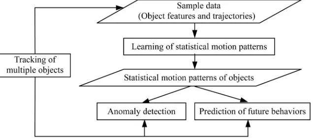
The automatically modeling of object behaviors without the assumption of any prior knowledge is an unsolved problem for current vision techniques. However, given a set of object trajectories, we can automatically construct statistical motion patterns, which are further used to detect anomalies and predict object future behaviors.

Fig. 1 gives an overview of our motion analysis system which is composed of four main modules: tracking of multiple objects, learning of statistical motion patterns, detection of anomalies, and prediction of future behaviors. The module for tracking multiple objects is implemented by clustering foreground pixels in each image frame and comparing pixel distributions between successive images. The outputs of this module are object trajectories and features (such as color, size, etc.). These outputs form the sample data for learning motion patterns. After enough sample data are acquired, object motion patterns are learned using a hierarchical trajectory clustering based on the fuzzyK-meansalgorithm. In the motion patterns, each pattern is represented by a chain of Gaussian distributions, and statistical descriptions of typical motion patterns are then formed. In the module for anomaly detection, we calculate the probabilities of the matching between ob-served behaviors and the learned motion patterns and then calculate the probability values of abnormality of the observed behaviors. In the module for behavior prediction, partial trajectories are matched to the learned motion patterns, and future behaviors are stochastically inferred.

4

T

M

O

tasks are based on the tracking of moving objects. In this paper, we focus on real traffic scenes where there are many vehicles and mutual occlusions between multiple vehicles. While there exist some algorithms [23], [24], [28], [31], [39], [51] for tracking multiple objects, most of them fail due to the complexity of motions in crowded traffic scenes. In this paper, a new fuzzy clustering-based tracking algorithm is proposed to robustly track multiple vehicles. This algorithm is based on the principle that a moving object is always associated with a cluster of pixels in the feature space and the features of each cluster change only slightly between consecutive frames [16], [38]. Fig. 2 illustrates the frame-work of our tracking algorithm. On the basis of background subtraction and feature extraction, a fast accurate fuzzy

K-means algorithm is used to cluster foreground pixels. Each cluster centroid corresponds to a moving object or a part of a moving object. The clustering results of the current frame, as the most important information, participate in the initialization of the cluster centroids of foreground pixels in the subsequent frame. A cluster centroidjin the subsequent frame and the cluster centroid in the current frame, which participates in the initialization of cluster centroid j, both correspond to the same object or the same part of an object. In the algorithm, clusters grow dynamically: They are created or are erased. A predication algorithm is used to integrate previous clustering results to ensure that the initial values of cluster centroids in the subsequent frame are close to the true object clusters.

4.1 Extraction of Foreground Pixels

In our clustering-based tracking algorithm, only the fore-ground pixels are clustered. Backfore-ground modeling and subtraction are performed to extract foreground pixels. The background image is updated by integrating the current imagecurrent into the current backgroundBcurrent:

Bupdated¼ ð1ÞBcurrentþcurrent, where Bupdated is the estimated background image and is an adaptation coefficient. By computing the difference between corre-sponding pixels incurrentandBcurrent, foreground pixels in the current frame are identified.

4.2 Acquisition of Pixel Features

In this algorithm, each foreground pixel is described with a feature vector f containing its coordinates ðx; yÞ, velocity

ðvx; vyÞ, and color in theRGB spaceðr; g; bÞ:f¼ ðx; y; wv

vx; wvvy; wcr; wcg; wcbÞ, where the weighting factorwc describes the relation between color and position, andwvthat between velocity and position. (In our experiments, we choose

wcto be 0.1 andwvto be 2 with the320240image size.) Compared with coordinate and color features, velocity features are difficult to acquire. Velocity can be estimated using an optical flow-based algorithm [3]. In our method, optical flow is computed by windowed correlation. For a foreground pixel p (p¼ ðx; yÞ) in the current frame and a foreground pixel p (p¼ ðx; yÞ) in the previous frame (p2RðpÞ, where RðpÞ is a search region around p), their dissimilarity is measured by:

Dðp; pÞ ¼ X

N

i¼N

XN

j¼N

Iðxþi; yþjÞ Iðxþi; yþjÞ

j j; ð1Þ

whereN defines the radius of the neighborhood patch of a pixel,I is the intensity in the current frame, and I _{is the}

intensity in the previous frame. Here, the Sum of Absolute Differences (SAD) is used to replace the correlation in [9], [27] due to the simplicity of implementation of SAD. Then, we find the pointp defined by:

p¼arg min

p_2RðpÞDðp; p

_{Þ: ð2Þ}

The optical flow at p can be estimated as p!p, and the

velocity ðvx; vyÞ can be described as the projection of the optical flow to thex,ycoordinate axes.

It is should be mentioned that a patch-based approach for optical flow estimation works well for patches containing “corner-like” intensities. In our experiments, a crowded traffic scene is considered where vehicles are relatively small and their constructions are complex. There exist “corner-like” intensities in the patches when the radius of the patches is properly selected. In addition, we only estimate the optical flow for foreground pixels. This greatly reduces the compu-tational cost, compared with the methods which estimate the optical flow for all pixels in the current frame.

4.3 Clustering of Foreground Pixels

After the pixel features are acquired, foreground pixels are clustered in the feature space. In order to improve the speed of the clustering process, we introduce a component quantization filtering to merge similar pixels. Then, the fuzzy K-means algorithm [1], [7], [13], [36] is applied to cluster merged foreground pixels.

4.3.1 Component Quantization Filtering

In component quantization filtering, the image plane is partitioned into square regions with equal size. The features in each square are represented by a “representative sample vector”Xiwhich is equal to the mean of the feature vectors of the foreground pixels in the region, and associated with a weightwi which is the number of foreground pixels in the region.

The component quantization filtering has the following functions:

. Some noisy samples are filtered out before clustering.

. The representative sample vectors fXig give a reduced and precise view of the original pixel feature data set.

4.3.2 FuzzyK-means Algorithm

The representative samples fXig are clustered using the weighting fuzzy K-means algorithm which is modified to support weighted feature vectors.

Let M denote the number of representative samples,N

the dimension of the representative sample vectors, andK

the number of cluster centroids. Cluster centroid j

(j¼1;. . .; K) is represented by an N-dimensional vector

Vj. In the first frame, the initial values (Vjð0Þ,1jK) of the cluster centroid vectors are randomly selected. In other frames, the values of Vjð0Þ are derived from the clustering results of the previous frames.

Given all representative sample vectorsfXlg(1lM), the degree of membershipRljof each samplelto each cluster centroidjis computed by:

Rlj¼

1= XlVj

2

PK m¼1

ð1= Xk lVmk2Þ

;1lM;1jK: ð3Þ

From (3), we can see that, the less the Euclidean distance between a sample and a cluster centroid, the more the membership of the sample to the cluster centroid.

According to the computed memberships, each cluster centroid vector is updated by:

Vjðtþ1Þ ¼VjðtÞ þ

PM l¼1

RljðtÞ wl ðXlVjðtÞÞ

PM l¼1

RljðtÞ wl

;1jK;

ð4Þ

where wl is the weight associated with representative sample vector l. From (4), we can see that, for a representative sample and a cluster centroid, the more their membership or the more weight associated with the sample, the more the sample contributes to the adjustment of the value of the cluster centroid vector.

It should be pointed out that in our algorithm the number of clusters is adjusted dynamically (see Section 4.4), making it possible to arrive at the correct number of clusters even when the number of clusters in the first frame is not correctly chosen.

4.4 Dynamic Growing of Cluster Centroids

Cluster centroids are created or erased as objects enter or leave the scene. This is called the dynamic growing of cluster centroids.

4.4.1 Creation of Cluster Centroids

In order to create cluster centroids, we manually define “entering regions” where objects enter the scene. Within each entering region, we find a subset of samples<where the Euclidean distance between each of these samples and its associated cluster centroidjexceeds a thresholdj. If the number of such samples is large enough to represent an object, a new entering event is detected. If the number of these samples can represent objects, new cluster centroids are created and trained using the sample set <. We use the information in the previous frame to evaluate the thresholdj. In the previous frame, we find the cluster centroid j _{corresponding to the cluster centroid j in the}

current frame and all samples best matching cluster centroid j_{. We calculate the Euclidean distances between}

these samples and cluster centroid j and select the maximum of these distances as thresholdj.

4.4.2 Erasure of Cluster Centroids

In order to implement the erasure of cluster centroids, we manually define “leaving regions” where objects leave the scene. Cluster centroid j is erased if the following two points are satisfied:

. The position of cluster centroidjis within a leaving region.

. The number of the samples corresponding to cluster centroidjis too small to represent the smallest object in the scene.

It is noted that manual definition of the entering or leaving regions increases the robustness of the cluster growing. Entering or leaving regions are not identified automatically using knowledge of the object positions in the image because 1) entering or leaving regions sometimes are not beside the image edges, for example, at the boundary of a static object such as a building and 2) even if these regions are beside the image edges, the decision as to whether an object is in one of the regions depends on a distance threshold which also should be defined manually.

4.5 Prediction of Cluster Centroids

For a cluster centroid in the current frame, a prediction algorithm is used to produce the initial value for the corresponding cluster centroid in the next frame. This prediction is based on information from current and previous frames about the cluster centroids which corre-spond to the same object or the same part of an object. This prediction not only expedites the convergence of the clustering process in the next frame, but it also ensures that each centroid in the current frame corresponds to a correct foreground pixel cluster in the next frame.

The Kalman filter is usually a good candidate for a prediction algorithm. In our work, many objects need to be tracked simultaneously, so there is a high computational cost. For this reason, we keep the computational cost of the tracking algorithm as small as possible. In order to decrease the computational cost, a fast prediction algorithm, the double exponential smoothing-based prediction algorithm [21], is selected. The running speed of the double exponential smoothing-based prediction algorithm is faster than that of the Kalman and extended Kalman filter-based predictors [21].

Given a cluster centroid vector at time t:ft

!

, its predictive value at time tþ is calculated from the following formulae:

f_t

! ¼ ft

!

þ ð1Þf_t!₁; ð5Þ

f_t

!

¼ f!_t þ ð1Þf_t!₁; ð6Þ

ftþ

!

¼ 2þ

ð1Þ

f_t

!

1þ

ð1Þ

f_t!₁; ð7Þ

wheref!_t smoothes the sequenceft

!

4.6 Modeling of Trajectories

In our algorithm, the successive cluster centroids which correspond to the same object or the same part of an object are connected to form a centroid trajectory. Of course, there may be objects which correspond to two or more cluster centroids in one frame. So, centroid trajectories should be grouped into object trajectories during the clustering. The centroid trajectories with the same motion constraint should be merged into one object trajectory. For two centroid trajectories, if they exist over the same sequence of frames, we calculate the distance between the two corresponding centroids in each frame. If the difference of these distances between any two successive frames is smaller than a threshold (which is set to 5 pixels in our experiments), the two centroid trajectories are merged. The merged trajectory is the mean of the centroid trajectories.

During tracking, we can also acquire object size, shape, texture, etc. In this paper, we select position, velocity, and size as features of an object in a frame and, thus, a trajectory which exists for n frames is represented as: T ¼ fF1; F2;. . .;

Fi;. . .; Fng, where Fi¼ ðxi; yi; vxi; vyi; sizeiÞ. Fi is called a

“point feature vector.”

4.7 Remark

From the above description of our tracing algorithm, we can see that, compared with traditional tracking algorithms, ours does not depend on accurate motion segmentation and complex matching between objects and motion regions. When partial occlusions between moving objects occur, these objects can still correspond to different cluster centroids due to the different features of the pixels corresponding to these objects. Prediction of cluster centroids ensures that each centroid corresponds to the correct object, even when this object is partially occluded. So, our tracking algorithm is robust for tracking multiple objects and, thus, suitable for crowded traffic scenes.

5

L

M

P

By tracking objects, a set of trajectories ¼ fT1;. . .;

Tl;. . .; TMg is acquired, where M denotes the number of sample trajectories andTlthelthtrajectory. These trajectories are used to learn object motion patterns ¼ f1;. . .;

j;. . .; Cg, whereCis the number of motion patterns, and

jis thejthmotion pattern. In this section, we describe the proposed learning algorithm, which includes hierarchical clustering of trajectories and acquisition of statistical motion patterns.

5.1 Hierarchical Clustering of Trajectories

The aim of clustering trajectories is to assign similar trajectories to the same cluster [33]. In order to handle a large number of trajectories, we hierarchically cluster trajectories according to different features. In our algorithm, the sample trajectories are clustered with two layers, as shown in Fig. 3. As trajectories belonging to different routes must be assigned to different clusters, in the first layer of clustering, sample trajectories are clustered into different routes according to trajectory spatial information. In the second layer of cluster-ing, trajectories belonging to the same route are further clustered according to temporal information.

5.1.1 Spatial-Based Clustering

In the spatial-based clustering (i.e., the first layer of clustering), all sample trajectories are input to the cluster-ing algorithm. In order to ensure the efficiency of the clustering, only coordinates of the points on each trajectory are kept for clustering, as coordinate information is enough to represent the spatial information of each trajectory. For each trajectory Tl, we construct an intermediate trajectory

T_l to represent the spatial information of trajectoryTl. We first cluster the intermediate trajectories using the fuzzy

K-means algorithm, and then cluster the original trajec-tories according to the their correspondences with the intermediate trajectories. Each intermediate trajectoryT_lis acquired through the following steps:

. Each intermediate trajectory T_l is a sequence of coordinates chosen from the original trajectoryTl. . Intermediate trajectories are resampled at larger time

intervals (once everytframes), i.e., we keep points in the intermediate trajectories at intervals oftframes, and remove those points between the kept points.

. Trajectories input to a clustering algorithm should have the same length (the same number of points). Each intermediate trajectory is linearly interpolated with points to ensure that all the intermediate trajectories have the same numberLof points. The set of the acquired intermediate trajectories is repre-sented by¼ fT₁;. . .; T_Mg.

In the fuzzyK-means-basedalgorithm for clustering the intermediate trajectories, each cluster centroid directly corresponds to a class of intermediate trajectories. Each cluster centroid is represented by a vector whose dimension is the same as the intermediate trajectories. The cluster centroid vectors are initialized randomly and adjusted gradually to form a mapping from input to output, which keeps the distribution features of the intermediate trajectories.

LetKdenote the number of cluster centroids andN the dimension of cluster centroid vectors. Cluster centroid j

(j¼1;. . .; K) is denoted by aN-dimensional vectorVj. For simplicity, each intermediate trajectoryT

l is represented by an N-dimensional vector Xl. The fuzzy membershipRlj of each sample l to each cluster centroid j (l¼1;2; ; M,

Vjðtþ1Þ ¼VjðtÞ þ

PM

l¼1RljðtÞ ðXlVjðtÞÞ

PM l¼1RljðtÞ

ð8Þ

until the following stability condition is satisfied:

max

1jK Vjðtþ1Þ VjðtÞ

< ": ð9Þ

Note that (8) is similar to (4) except that the weight term in (4) representing the number of pixels in a representative sample vector is absent in (8).

The quality of clustering results is automatically measured using the Tightness and Separation Criterion [48] (TSC):

T SCðV ; KÞ ¼

1 M

PK j¼1

PM

l¼1R2ljXlVj

2

minj1;j2Vj1Vj2

2 : ð10Þ

The criterionT SCðV ; KÞis the ratio of the mean of the square of the distance between each input sample and its corre-sponding cluster centroid, to the minimum distance between any two cluster centroids. The clustering result should make the distances between the cluster centroids as large as possible, and the distance between an input sample and its corresponding cluster centroid as small as possible. We estimate the number of cluster centroids by checking whether

T SCðV ; KÞcan be reduced by increasing or decreasing the number of cluster centroids. The estimated number of clusters corresponds to the minimum ofT SCðV ; KÞ.

In addition, the minimum number of samples corre-sponding to a cluster centroid is specified as a parameter for the clustering algorithm. If a cluster contains less than the required minimum number of samples, the cluster is merged into its nearest neighboring cluster. This avoids that the clustered results overfit some samples.

Corresponding to the clustering result of the intermedi-ate trajectories, the set of original trajectories ¼ fT1;. . .; TMgis clustered intoK subsets:

¼ffT1;1;. . .; T1;M1g;. . .;

fTi;1;. . .; Ti;Mig;. . .;fTK;1;. . .; TK;MKgg;

ð11Þ

whereMidenotes the number of original trajectories in the

ithsubset. The trajectories in each subset correspond to the same cluster of intermediate trajectories.

In the following, each subset i¼ fTi;1;. . .; Ti;Mig is

further clustered using temporal information.

5.1.2 Temporal-Based Clustering

The scale of each subset i is much less than that of the whole sample trajectories, so temporal information is introduced to further cluster each subset of trajectories.

In order to cluster the subseti, additional point feature vectors are padded to each trajectoryTli in i to obtain an

intermediate trajectory T_li which has a fixed length L_i . Suppose that trajectory Tli has n point feature vectors and

the lengthL_i corresponds togpoint feature vectors. Then,

gn feature vectors with 0 velocity are padded to Tli to

produce T_l

i withgpoint feature vectors. The influence of

this padding can be ignored. At the current research stage, better methods have not been found.

By this padding, each subset i yields a set i of intermediate trajectories. These intermediate trajectories are clustered using the fuzzyK-meansalgorithm. The clustering procedures are the same as the spatial-based clustering. The

number of cluster centroidsKifor the seti is also estimated by minimizing the right-hand side of (10). Accordingly, intermediate trajectories ini are clustered intoKiclusters. Abnormal trajectories may exist in the sample trajectories. As abnormal behaviors rarely occur in the scene, a cluster which contains few sample trajectories may correspond to an abnormal behavior pattern. Such clusters are removed. So, in our method, it is not necessary to ensure that all the sample trajectories are normal.

After the temporal-based clustering, all intermediate trajectories are clustered intoC clusters. According to the correspondence between the original trajectories and the intermediate trajectories, the original trajectories are clus-tered intoCsets of trajectories:

¼ ffT1;1;. . .; T1;M1g;. . .;

fTj;1;. . .; Tj;Mjg;. . .;fTC;1;. . .; TC;MCgg;

ð12Þ

whereMjdenotes the number of the original trajectories in thejthtrajectory subset.

In the following, each trajectory subset j¼

fTj;1;. . .; Tj;Mjg is described as a motion pattern j.

5.2 Statistical Motion Patterns

Each motion pattern j is represented by a chain of ‘j probability distributions f’j;1; ’j;2;. . .; ’j;i;. . .; ’j;‘jg. Each

probability distribution in motion patternjcorresponds to

j successive point feature vectors in a sample trajectory. LetLj be the maximum length of all trajectories inj. The relationship between ‘j and j is j¼ Lj=‘j

. j is an integer which is no less than 1. In our method, each probability distribution in a motion pattern corresponds to more than one point feature vectors in a trajectory. This makes the motion pattern more flexible to adapt the object position alteration along the moving direction.

In the paper, each probability distribution’j;iis assumed to be Gaussian. Letandbe, respectively, the mean and the covariance matrix of’j;i. We find the corresponding point feature vectors in the sample trajectories injto estimate the parameters of’j;i:and. Letk¼ ði1Þjþ1and

#¼ ij if i < ‘j

Lj if i¼‘j:

ð13Þ

Then, point feature vectorsFk; Fkþ1;. . .; F# in each sample trajectory injare used to estimate the parameters of ’j;i. According to the maximum likelihood evaluation, the following formulae are obtained:

¼ 1 Mið#kþ1Þ

PMi

i¼1 P# m¼k

Fi;m

¼ 1

Mið#kþ1Þ PMi

i¼1 P# m¼k

Fi;m Fi;m T : 8 > > > < > > > :

ð14Þ

Accordingly, the probability (rather than probability den-sity) of a point Z under probability distribution ’j;i is specified by:

PðZj’j;iÞ ¼exp 1 2ðZÞ

T1

ðZÞ

: ð15Þ

motion pattern j, we define the mean of the Euclidean distance betweenT and the mean ofjas:

dðT ; jÞ ¼ 1

L

ffiffiffiffiffiffiffiffiffiffiffiffiffiffiffiffiffiffiffiffiffiffiffiffiffiffiffiffiffiffiffiffiffiffiffiffiffiffiffi XL

i¼1

ðFi_{j; i=d jeÞ}2

v u u

t ; ð16Þ

where_{j; i=}

j

d e is the mean of’j; i=d je. The random variable

dðT ; jÞ approximately obeys the exponential distribution with a parameter and the probabilityPðTjjÞis estimated as:

PðTjjÞ ¼e dðT ;jÞ: ð17Þ We calculate the meandkof the Euclidean distance between each sample trajectorykinjand the mean ofj. According to the maximal likelihood evaluation, parameter is estimated as:

¼Pnn k¼1dk

; ð18Þ

wheren is the number of trajectories inj.

In addition, the probabilities of all sample trajectories inj under j are used to evaluate the optimal value of the coefficientj. If the sum of these probabilities can be increased with increase or decrease ofj,jis increased or decreased.

It should be pointed out that a motion pattern described above is similar to a Left-to-Right HMM. As the lengths of different trajectories change greatly, different numbers of states in HMMs should be used to represent change of trajectory lengths. It is demanding how the numbers of states are automatically estimated and how such HMMs are used to incrementally detect anomalies and implement long-time prediction.

5.3 Remark

Compared with the motion patterns in existing approaches for learning motion patterns, our motion patterns have the following advantages:

. Behaviors represented by trajectories are intuitively and statistically modeled.

. Positions in trajectories are modeled using prob-ability distributions with alterable covariance values.

. The sequential order of trajectory points linked at uniform time intervals is directly modeled.

Compared with previous approaches for learning motion patterns, our approach has following advantages:

. The number of motion patterns is estimated rather than assumed.

. Abnormal trajectories are allowed to exist in the sample trajectories.

. The fuzzy K-means clustering in our approach is superior to vector quantization clustering used in previous work [19], [20], [42], [43], on the condition that online learning is not concerned.

6

A

D

B

P

After motion patterns are obtained, we can use them to incrementally detect anomalies, judge whether or not an observed trajectory is abnormal, and predict the future

trajectory along which an object is going to move according to the current partially observed trajectory.

6.1 Anomaly Detection

6.1.1 Incremental Detection of Anomalies

The aim of incremental detection of anomalies is to detect object motion anomalies as soon as they occur. LetTbe the

observed part of an object trajectory. Suppose that there are

k sample points in T. We decide whether an anomaly

occurs when the object arrives at current positionk. We first calculate the probability of trajectoryT under

each motion patternj in the same way as formulated by (16), (17), and (18). According to the Bayes rule, the probability ofjgivenT is calculated by:

PðjjTÞ ¼

PðTjjÞPðjÞ

PC m¼1

PðTjmÞPðmÞ

; j¼1;2; ; C; ð19Þ

where PðjÞ is estimated by the ratio of the number of samples corresponding toj to the number of all samples. We find the patternj to whichTcorresponds by:

j¼arg max

j PðjjTÞ: ð20Þ Then, we calculate the probability of the pointkunder the

k=j

thprobability distribution’_{j; k=}

j

d e:PðFkj’j; k=d jeÞ.

The probability of anomaly occurrence when the object arrives at pointkis represented by:

AðkÞ ¼1PðFkj’j; k=d jeÞ: ð21Þ

If probabilityAðkÞis big enough, an anomaly is considered to potentially occur when the object arrives at pointk. When a serial of such unusual points are detected, an anomaly is marked. In this way, the dependence of the incremental anomaly detection on the tracker is decreased.

6.1.2 Detection of Abnormal Trajectories

It is also interesting to evaluate the abnormality of a complete trajectory. Given a trajectoryT ¼ ðF1; F2;. . .; FnÞ, we calculate the probability ofT under each motion pattern and look for the motion patternj that has the maximum

likelihood with trajectoryT:

j¼arg max

j PðTjjÞ: ð22Þ If the probabilityPðTjjÞofTunder the motion patternjis

less than a thresholdj, the trajectory is treated as abnormal.

We use the probability of each of the samples which correspond toj given motion patternj to calculate the

thresholdj. For each of these samplesTl, we calculate the

probabilityPðTljjÞofTlunder motion patternj. We take

the minimum of allPðTljjÞas the thresholdj:

j¼min

l PðTljjÞ: ð23Þ In this way, each motion pattern has a threshold. So, we can acquire a threshold set:f1;2;. . .;Cg.

6.2 Behavior Prediction

Future motion of an object can be predicted using the learned motion patterns. Let T be the initial part of a

The probabilityPðTjjÞofTunder each motion patternj is calculated in the same way as formulated by (16), (17), and (18). According to the Bayes rule, the probability

PðjjTÞ of j given T is calculated using the formula

similar to (19).PðjjTÞis just the probability that the object

is expected to move along the trajectory represented by motion patternj. The trajectory represented by the motion pattern with the highest probability is chosen as the most probable one along which the object is expected to move. If

PðjjTÞis very small,jis rejected as a possible trajectory for the object.

7

E

R

All the above algorithms are implemented using Visual C++6.0 on the Windows XP platform. In the following, tracking results are first introduced. Performance of the algorithm for learning motion patterns is then evaluated. Finally, the results of anomaly detection and behavior prediction are demonstrated.

7.1 Tracking

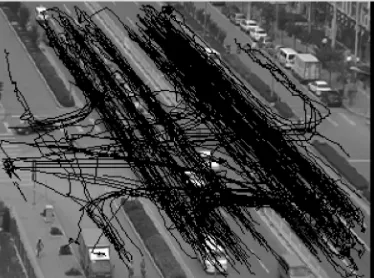
In order to verify the accuracy and robustness of the proposed tracking algorithm, we tested it in a crowded traffic intersec-tion scene. Fig. 4 shows three examples of pixel segmentaintersec-tion and clustering. The images are of size320240pixels. Fig. 5 illustrates the extracted trajectories. In the testing time interval, partial occlusions between moving vehicles and those between moving vehicles and static street attachments such as street lamps and trees occur frequently. The correctness of the tracking results is checked by our own visual judgment. During the testing time interval, 1,216 mo-tion trajectories were produced using our tracking algorithm. Also, 1,184 motion trajectories were seen to be correct. So, the

correct rate of tracking during this time interval is 97.4 percent. This indicates that the proposed tracking algorithm is suitable for traffic surveillance. The major reason why 2.6 percent trajectories are unacceptable is local disturbances from groups of pedestrians and long lasting or serious occlusions between moving vehicles.

Fig. 6 shows computational costs in three key parts in the proposed tracking algorithm: the fast fuzzyK-means algo-rithm, optical flow estimation, and the growing and predic-tion of cluster centroids. In this paper, all values of running time are calculated on a P4 1.8GHz computer. From Fig. 6, we can see that our tracker runs at the speed of 5-10 frames in a second with a moderate number of vehicles present in the scene. As the number of vehicles increases, the running cost does not quickly increase.

Since anomalies do not always occur in real world scenes, in order to test the performance of our anomaly detection approach, we also experimented with an indoor model simulating a real traffic scene (as shown in Fig. 7). The model is of size 2:4m2:4m. The model includes crossroads, parking lots, one-way roads, and multilane roads, etc., and Fig. 4. Examples of tracking results.

Fig. 5. Trajectories from real scene.

Fig. 6. Computational cost.

also involves many events such as turning left, turning right, entering, and leaving. The model also includes radio-controlled toy cars. By driving the toy cars, we can acquire a series of trajectories. Fig. 8 shows 400 trajectories acquired by tracking the toy cars. As the indoor model scene is comparatively ”clean,” the trajectories are smoother than those from the real traffic scene.

7.2 Learning of Motion Patterns

Figs. 9 and 10 show the learning results, respectively, in the model traffic scene and in the real traffic scene using our algorithm. In the figures, a white line represents the mean of a motion pattern. As shown in the figures, the learned motion patterns are consistent with the sample trajectories, so the results can be treated as satisfactory.

Fig. 11 shows four motion patterns and the correspond-ing sample trajectories in the model traffic scene. Fig. 12 shows three motion patterns and the corresponding sample trajectories in the real traffic scene. In the shown motion patterns, the middle lines represent the means of the Gaussian distributions and shadows standard deviations. From these figures, we can see that the motion patterns well reflect the distributions of the sample trajectories.

In the following, the fuzzy K-means-based learning method is compared with the vector quantization-based method used in [19], [20], [42], [43]. The most convincing comparison is to determine how well the algorithm does versus ground truth labeled by hand. However, it is difficult to manually label a large set of samples. So, we use the Tightness and Separation Criterion (TSC) [48] to automatically measure the validity of the clustering results. Tables 1 and 2 demonstrate theTSCof the two learning algorithms, respectively, for the model scene and the real traffic scene with different stability conditions. For each stability condition, the experiment was performed for three times with different initial weights. From Tables 1 and 2, we see that, with the same stability condition, the values of criterionTSCof the fuzzyK-meansalgorithm are much less Fig. 8. Trajectories from model scene.

Fig. 9. Learned result in model scene.

Fig. 10. Learned result in real traffic scene.

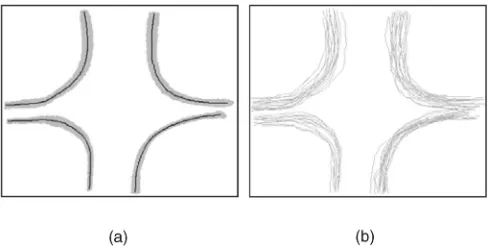
Fig. 11. Four motion patterns in model scene: (a) Motion patterns. (b) Sample trajectories.

Fig. 12. Three motion patterns in real traffic scene: (a) Motion patterns. (b) Sample trajectories.

TABLE 1

than those of the vector quantization algorithm. Extensive experiments show that the fuzzy K-means algorithm has more efficient learning results.

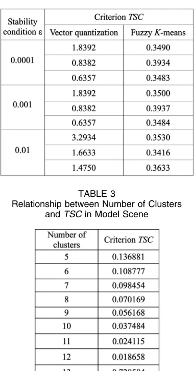
Table 3 shows the relationship between the number of clusters and the criterionTSCin the spatial-based clustering of the sample trajectories from the model scene. We can see, from Table 3, that the criterion TSC decreases when the number of clusters increases from 5 to 12, but dramatically increases when it is equal to 13. So, it is proper to select the number of clusters as 12 in the spatial-based clustering. This result is consistent with the scene. As shown in Figs. 7 and 8,

there are four entrances by which vehicles enter the scene: “left,” “bottom,” “right,” and “top.” Corresponding to each entrance, there are three routes along which vehicles can move: “turn left,” “go ahead,” and “turn right.” Thus, there are 12 actual routes in the scene, and this result is reflected in the values ofTSC. The final learned motion patterns shown in Fig. 9 are acquired by, using the temporal-based clustering, further clustering trajectories assigned to each route.

For the real traffic scene, by the spatial-based clustering, all trajectories are clustered into 18 clusters (i.e., 18 subsets of trajectories corresponding to 18 routes). Table 4 shows the relationship between the number of clusters and the criterion TSC, when one of the subsets of trajectories is further clustered using the temporal-based clustering. We can see, from Table 4, that the value ofTSCdecreases when the number of cluster increases from 5 to 10, but increases when it is equal to 11. So, it is proper to select the number of clusters as 10 for clustering this subset of trajectories. The final learned motion patterns shown in Fig. 10 are acquired by further clustering all the subsets of trajectories.

7.3 Anomaly Detection

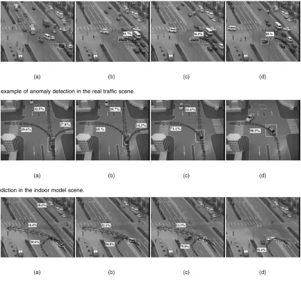
With the learned motion patterns, we can use the method introduced in Section 6.1.1 to incrementally find anomalies and use the method introduced in Section 6.1.2 to detect abnormal trajectories. The correctness of the following anomaly detection results is verified by our visual judgment. Fig. 13 is an example of anomaly detection in the indoor model scene. The trajectory of the car is shown as a series of arrows, with the size of the arrowhead representing the speed of the car. Each abnormal point is marked with an “x” sign at the center of the arrowhead. The abnormality probability is

TABLE 2

Performance Comparison in Real Traffic Scene

TABLE 3

Relationship between Number of Clusters andTSCin Model Scene

TABLE 4

Relationship between Number of Clusters and

TSCin Real Scene

shown beside the car. The car entered the scene from the bottom and then turned right. At the beginning, the car moved within the normal lane, as shown in Fig. 13a. Then, it entered the region (a grassplot) where admission is forbid-den, as shown in Figs. 13b, 13c, and 13d. Several abnormal points are therefore detected.

Fig. 14 illustrates another example of anomaly detection in the real crowded traffic scene. In the right-bottom corner of the scene, there are three lanes, separated with white mark lines, along which vehicles can run upward. Only along the left lane can vehicles turn left or turn around. A car entered the scene along the middle lane along which all vehicles are required to run ahead, as shown in Fig. 14a. However, the car then made a “U” turn along the lane. This is a serious traffic offense, which is correctly detected as shown in Figs. 14b, 14c, and 14d.

7.4 Behavior Prediction

Fig. 15 shows an example of prediction in the indoor model scene. The percentage beside a trajectory represents the probability with which the car is expected to move along the trajectory. The car entered the scene from the bottom and then turned left. Fig. 15a shows the three most probable trajectories which the car might follow; in Fig. 15b, the

probability values with which the car would move along these three trajectories are changed; in Fig. 15c, the right-turn trajectory is eliminated because the probability of the car making a right turn has become very small. In Fig. 15d, the forward trajectory is also removed for the same reason.

Another similar example of behavior prediction in the real traffic scene is demonstrated in Fig. 16. A car entered the scene from the right-bottom corner. Initially, it had three potential moving ways: moving ahead, turning left, and turning around, as shown in Fig. 16a. During the motion, it tended to turn left or turn around, as shown in Fig. 16b and Fig. 16c. After further motion, its tendency to turn around became clear, as shown in Fig. 16d.

Both examples in Figs. 15 and 16 show that the predictions are consistent with one’s visual judgment, demonstrating the good accuracy of the algorithm in predicting object behaviors.

7.5 Remark

The above describes the performance of our system. Certainly, our system has limitations:

. Entering and leaving regions are defined manually for tracking multiple objects.

Fig. 14. An example of anomaly detection in the real traffic scene.

Fig. 15. Prediction in the indoor model scene.

. Online learning of motion patterns is not considered.

. Incremental detection of anomalies is dependent on robustness of tracking.

8

D

C

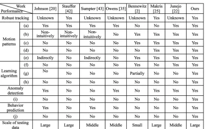
In the introduction, we have reviewed in detail the recent work on learning motion patterns. Table 5 compares our work with previous ones. In contrast with Johnson and Hogg [20], Sumpter and Bulpitt [43], Makris and Ellis [25], and Junejo et al. [22], our work has introduced probability distributions to the motion patterns; the number of motion patterns is evaluated; and anomaly detection and behavior prediction are implemented based on statistical theory. In contract with Stauffer and Grimson [42], we have intuitively modeled the linking relationship between successive points in a trajectory and implemented anomaly detection and behavior prediction. Compared with Owens and Hunter [35], we have constructed motion patterns represented by trajectories rather than only point distributions and im-plemented the detection of abnormal behaviors represented by complete trajectories and behavior prediction. Com-pared with Bennewitz et al. [2], we have modeled trajectories sampled at uniform time intervals, made the covariance alterable, used a large data set to test our learning algorithm, and implemented anomaly detection and long-term prediction.

In addition, our system for learning motion patterns is based on the robust tracking of multiple objects. Our

tracking algorithm is not dependent on accurate motion segmentation and it does not require complex matching between objects and motion regions.

In summary, our system for learning motion patterns has many advantages, and it has solved many issues left in previous work, such as representation of a motion pattern with probability distributions with alterable covariance values, estimation of the number of motion patterns, processing of abnormal trajectories in the sample set, and usage of the detection probability theory to identify anomalies and predict future behaviors.

Our future work will focus on the following aspects:

. We will model the behavior of “stop” in our motion patterns.

. We will attach semantic meanings to motion patterns using stochastic grammars [18], [30] or the Past-Now-Future Networks (PNF) [40].

. We will apply the methods for automatically extracting the rules explaining the phenomena hidden in the input data to behavior analysis.

. We will introduce motion patterns for interactions between objects.

A

This work is partly supported by NSFC (Grant No. 60373046 and 60520120099) and the Natural Science Foundation of Beijing (Grant No. 4041004).

TABLE 5

Comparison of the Work of Learning Motion Patterns

R

[1] A. Baraldi and P. Blonda, “A Survey of Fuzzy Clustering Algorithms for Pattern Recognition—Part II,”IEEE Trans. Systems, Man, and Cybernetics—Part B: Cybernetics,vol. 29, no. 6, pp. 786-801, 1999.

[2] M. Bennewitz, W. Burgard, and G. Cielniak, “Utilizing Learned Motion Patterns to Robustly Track Persons,”Proc. Joint IEEE Int’l Workshop Visual Surveillance and Performance Evaluation of Tracking and Surveillance,pp. 102-109, Oct. 2003.

[3] M.J. Black and P. Anandan, “A Framework for the Robust Estimation of Optical Flow,” Proc. Int’l Conf. Computer Vision,

pp. 231-236, 1993.

[4] A.F. Bobick and A.D. Wilson, “A State-Based Technique to the Representation and Recognition of Gesture,”IEEE Trans. Pattern Analysis and Machine Intelligence,vol. 19, no. 12, pp. 1325-1337, Dec. 1997.

[5] M. Brand, “Understanding Manipulation in Video,” Proc. Int’l Conf. Automatic Face and Gesture Recognition,pp. 94-99, 1996.

[6] M. Brand and V. Kettnaker, “Discovery and Segmentation of Activities in Video,” IEEE Trans. Pattern Analysis and Machine Intelligence,vol. 22, no. 8, pp. 844-851, Aug. 2000.

[7] J.F. Colen and T. Hutcheson, “Reducing the Time Complexity of the Fuzzy C-Means Algorithm,”IEEE Trans. Fuzzy Systems,vol. 2, no. 2, pp. 263-267, 2002.

[8] R.T. Collins, A.J. Lipton, T. Kanade, H. Fujiyoshi, D. Duggins, Y. Tsin, D. Tolliver, N. Enomoto, O. Hasegawa, P. Burt, and L. Wixson, “A System for Video Surveillance and Monitoring,” Technical Report CMU-RI-TR-00-12, Robotics Inst., Carnegie Mellon Univ., May 2000.

[9] R. Cutler and M. Turk, “View-Based Interpretation of Real-Time Optical Flow for Gesture Recognition,” Proc. IEEE Int’l Conf. Automatic Face and Gesture Recognition,pp. 416-421, 1998.

[10] L. Davis, S. Fejes, D. Harwood, Y. Yacoob, I. Hariatoglu, and M.J. Black, “Visual Surveillance of Human Activity,”Proc. Asian Conf. Computer Vision,vol. 2, pp. 267-274, 1998.

[11] T.V. Duong, H.B. Bui, D.Q. Phung, and S. Venkatesh, “Activity Recognition and Abnormality Detection with the Switching Hidden Semi-Markov Model,” Proc. IEEE Conf. Computer Vision and Pattern Recognition,vol. I, pp. 838-845, June 2005.

[12] T. Ellis, D. Makris, and J. Black, “Learning a Multi-Camera Topology,”Proc. Joint IEEE Int’l Workshop VS-PETS,pp. 165-171, Oct. 2003.

[13] S. Eschrich, J. Ke, L.O. Hall, and D.B. Goldgof, “Fast Accurate Fuzzy Clustering Through Data Reduction,” IEEE Trans. Fuzzy Systems,vol. 11, no. 2, pp. 262-270, 2003.

[14] A. Galata, N. Johnson, and D. Hogg, “Learning Variable-Length Markov Models of Behavior,”Computer Vision and Image Under-standing,vol. 81, no. 3, pp. 398-413, 2001.

[15] I. Haritaoglu, D. Harwood, and L.S. Davis, “W4_{: Real-Time}

Surveillance of People and Their Activities,”IEEE Trans. Pattern Analysis and Machine Intelligence,vol. 22, no. 8, pp. 809-830, Aug. 2000.

[16] B. Heisele, U. KreBel, and W. Ritter, “Tracking Nonrigid, Moving Objects Based on Color Cluster Flow,”IEEE Conf. Computer Vision and Pattern Recognition,pp. 257-260, 1997.

[17] W.M. Hu, T.N. Tan, L. Wang, and S.J. Maybank, “A Survey on Visual Surveillance of Object Motion and Behaviors,”IEEE Trans. Systems, Man, and Cybernetics, Part C: Applications and Reviews,

vol. 34, no. 3, pp. 334-352, 2004.

[18] Y.A. Ivanov and A.F. Bobick, “Recognition of Visual Activities and Interactions by Stochastic Parsing,”IEEE Trans. Pattern Analysis and Machine Intelligence,vol. 22, no. 8, pp. 852-872, Aug. 2000.

[19] N. Johnson, “Behaviour Model and Analysis,” PhD Thesis, Univ. of Leeds, 1999.

[20] N. Johnson and D. Hogg, “Learning the Distribution of Object Trajectories for Event Recognition,”Image and Vision Computing,

vol. 14, no. 8, pp. 609-615, 1996.

[21] J. Joseph and J. Laviola, “Double Exponential Smoothing: An Alternative to Kalman Filter-Based Predictive Tracking,” Proc. Conf. Immersive Projection Technology and Virtual Environments 2003,pp. 199-206, 2003.

[22] I.N. Junejo, O. Javed, and M. Shah, “Multi Feature Path Modeling for Video Surveillance,”Proc. Int’l Conf. Pattern Recognition,vol. 2, pp. 716-719, 2004.

[23] S. Kamijo, Y. Matsushita, K. Ikeuchi, and M. Sakauchi, “Traffic Monitoring and Accident Detection at Intersections,”IEEE Trans. Intelligent Transportation Systems,vol. 1, no. 2, pp. 108-118, 2000.

[24] D. Koller, J. Weber, and J. Malik, “Robust Multiple Car Tracking with Occlusion Reasoning,”Proc. European Conf. Computer Vision,

pp. 189-196, 1994.

[25] D. Makris and T. Ellis, “Learning Semantic Scene Models from Observing Activity in Visual Surveillance,”IEEE Trans. Systems, Man, and Cybernetics—Part B,vol. 35, no. 3, pp. 397-408, 2005.

[26] D. Makris and T. Ellis, “Path Detection in Video Surveillance,”

Image and Vision Computing,vol. 20, no. 12, pp. 895-903, 2002.

[27] B. Maurin, O. Masoud, and N. Papanikolopoulos, “Monitoring Crowded Traffic Scenes,” Proc. IEEE Int’l Conf. Intelligent Transportation Systems,pp. 19-24, 2002.

[28] S. McKenna, S. Jabri, Z. Duric, A. Rosenfeld, and H. Wechsler, “Tracking Groups of People,”Computer Vision and Image Under-standing,vol. 80, no. 1, pp. 42-56, 2000.

[29] U. Meier, R. Stiefelhagen, J. Yang, and A. Waibel, “Towards Unrestricted Lip Reading,”Int’l J. Pattern Recognition and Artificial Intelligence,vol. 14, no. 5, pp. 571-585, Aug. 2000.

[30] D. Minnen, I. Essa, and T. Starner, “Expectation Grammars: Leveraging High-Level Expectations for Activity Recognition,”

Proc. IEEE Conf. Computer Vision and Pattern Recognition,vol. 2, pp. 626-632, June 2003.

[31] A. Mittal and L.S. Davis, “M2Tracker: A Multi-View Approach to Segmenting and Tracking People in a Cluttered Scene,” Int’l J. Computer Vision,vol. 51, no. 3, pp. 189-203, Feb./Mar. 2003.

[32] N.T. Nguyen, H.H. Bui, S. Venkatesh, and G. West, “Recognising and Monitoring High-Level Behaviours in Complex Spatial Environments,” Proc. IEEE Conf. Computer Vision and Pattern Recognition,vol. 2, pp. 620-625, June 2003.

[33] W.M. Hu, D. Xie, T.N. Tan, and S. Maybank, “Learning Patterns of Activity Using Fuzzy Self-Organizing Neural Network,” IEEE Trans. Systems, Man, and Cybernetics—Part B, vol. 34, no. 3, pp. 1618-1626, June 2004.

[34] N.M. Oliver, B. Rosario, and A.P. Pentland, “A Bayesian Computer Vision System for Modeling Human Interactions,”

IEEE Trans. Pattern Analysis and Machine Intelligence,vol. 22, no. 8, pp. 831-843, 2000.

[35] J. Owens and A. Hunter, ”Application of the Self-Organizing Map to Trajectory Classification,” Proc. IEEE Int’l Workshop Visual Surveillance,pp. 77-83, 2000.

[36] N.R. Pal and J.C. Bezdek, “Complexity Reduction for Large Image Processing,”IEEE Trans. Systems, Man, and Cybernetics—Part B,

vol. 32, no. 5, pp. 598-611, 2002.

[37] S. Park and J.K. Aggarwal, “Semantic-Level Understanding of Human Actions and Interactions Using Event Hierarchy,”Proc. IEEE Conf. Computer Vision and Pattern Recognition Workshop,

pp. 12-12, 2004.

[38] A.E.C. Pece, “From Cluster Tracking to People Counting,”Proc. IEEE Workshop Performance Evaluation of Tracking and Surveillance,

pp. 9-17, June 2002.

[39] N. Peterfreund, “Robust Tracking of Position and Velocity with Kalman Snakes,” IEEE Trans. Pattern Analysis and Machine Intelligence,vol. 21, no. 6, pp. 564-569, June 1999.

[40] C.S. Pinhanez, “Representation and Recognition of Action in Interactive Spaces,” PhD thesis, MIT Media Laboratory, 1999.

[41] T. Starner, J. Weaver, and A. Pentland, “Real-Time American Sign Language Recognition Using Desk and Wearable Computer-Based Video,”IEEE Trans. Pattern Analysis and Machine Intelligence,

vol. 20, no. 12, pp. 1371-1375, Dec. 1998.

[42] C. Stauffer and W.E.L. Grimson, “Learning Patterns of Activity Using Real-Time Tracking,” IEEE Trans. Pattern Analysis and Machine Intelligence,vol. 22, no. 8, pp. 747-757, Aug. 2000.

[43] N. Sumpter and A. Bulpitt, “Learning Spatio-Temporal Patterns for Predicting Object Behavior,” Image and Vision Computing,

vol. 18, no. 9, pp. 697-704, 2000.

[44] C. Town, “Ontology-Driven Bayesian Networks for Dynamic Scene Understanding,” Proc. IEEE Conf. Computer Vision and Pattern Recognition Workshops,pp. 124-124, 2004.

[45] N. Vaswani, A.R. Chowdbury, and R. Chellappa, “Activity Recognition Using the Dynamics of the Configuration of Interact-ing Objects,” Proc. IEEE Conf. Computer Vision and Pattern Recognition,vol. 2, pp. 633-640, 2003.

[47] A.D. Wilson, A.F. Bobick, and J. Cassell, “Temporal Classification of Natural Gesture and Application to Video Coding,”Proc. IEEE Conf. Computer Vision and Pattern Recognition,pp. 948-954, 1997.

[48] X. Xie and G. Beni, “A Validity Measure for Fuzzy Clustering,”

IEEE Trans. Pattern Analysis and Machine Intelligence,vol. 13, no. 8, pp. 841-847, Aug. 1991.

[49] Y. Yacoob and M. Black, “Parameterized Modeling and Recogni-tion of Activities,”Proc. Int’l Conf. Computer Vision,pp. 120-127, 1998.

[50] M.-H. Yang, N. Ahuja, and M. Tabb, “Extraction of 2D Motion Trajectories and Its Application to Hand Gesture Recognition,”

IEEE Trans. Pattern Analysis and Machine Intelligence,vol. 24, no. 8, pp. 1061-1074, Aug. 2002.

[51] T. Zhao and R. Nevatia, ”Bayesian Human Segmentation in Crowded Situations,”Proc. IEEE Int’l Conf. Computer Vision and Pattern Recognition,vol. 2, pp. 459-466, July 2003.

[52] H. Zhong, J. Shi, and M. Visontai, “Detecting Unusual Activity in Video,” Proc. IEEE Int’l Conf. Computer Vision and Pattern Recognition,vol. 2, pp. 819-826, June-July 2004.

[53] D. Xie, W. Hu, T. Tan, and J. Peng, “A Multiobject Tracking System for Surveillance Video Analysis,”Proc. Int’l Conf. Pattern Recognition,pp. 767-770, 2004.

Weiming Hureceived the PhD degree from the Department of Computer Science and Engineer-ing, Zhejiang University. From April 1998 to March 2000, he was a postdoctoral research fellow with the Institute of Computer Science and Technology, Founder Research and Design Center, Peking University. Since April 1998, he has been with the National Laboratory of Pattern Recognition, Institute of Automation, Chinese Academy of Sciences. Now, he is a professor and a PhD student supervisor in the lab. His research interests are in visual surveillance, neural networks, filtering of Internet objectionable information, retrieval of multimedia, and understanding of Internet behaviors. He has published more than 70 papers on national and international journals and international conferences.

Xuejuan Xiaoreceived the BSc degree in the Special Class for Gifted Young from the Uni-versity of Science and Technology of China (USTC), Hefei, China, in 2002. In 2005, she received the MS degree at the National Labora-tory of Pattern Recognition, Institute of Automa-tion, Chinese Academy of Sciences, Beijing. Her research interests include pattern recognition and computer vision.

Zhouyu Fureceived the BSc degree in informa-tion engineering from Zhejiang University, Chi-na, in 2001 and the MSc degree in pattern recognition from the National Laboratory of Pattern Recognition, Institute of Automation, Chinese Academy of Sciences, China, in 2004. He is currently a PhD candidate in the Depart-ment of Information Engineering, Research School of Information Sciences and Engineer-ing, Australian National University, Australia. His research interests include pattern recognition and computer vision.

Dan Xiereceived the BS degree in automatic control from the Beijing University of Aeronau-tics and AstronauAeronau-tics (BUAA), Beijing, China, in 2001. He received the MS degree at BUAA, in 2004. He is a PhD Candidate in the Computer Science Department, the University of Massa-chusetts, Amherst. His current research inter-ests include pattern recognition, machine learning, and neural networks.

Tieniu Tanreceived the BSc degree in electro-nic engineering from Xi’an Jiaotong University, China, in 1984 and the MSc, DIC, and PhD degrees in electronic engineering from the Imperial College of Science, Technology and Medicine, London, United Kingdom, in 1986, 1986, and 1989, respectively. He joined the Computational Vision Group, Department of Computer Science, The University of Reading, England, in October 1989, where he worked as a research fellow, senior research fellow, and lecturer. In January 1998, he returned to China to join the National Laboratory of Pattern Recognition, the Institute of Automation of the Chinese Academy of Sciences, Beijing. He is currently a professor and the director of the National Laboratory of Pattern Recognition as well as president of the Institute of Automation. His current research interests include image processing, computer vision, pattern recognition, and robotics. He is an associate editor ofPattern Recognitionand of theIEEE Transactions on Pattern Analysis and Machine Intelligence. He is a fellow of the IEEE.

Steve Maybank received the BA degree in mathematics from King’s College Cambridge in 1976 and the PhD degree in computer science from Birkbeck College, University of London in 1988. He joined the Pattern Recognition Group at Marconi Command and Control Systems, Frimley, in 1980 and moved to the GEC Hirst Research Centre, Wembley, in 1989. From 1993-1995, he was a Royal Society/EPSRC Industrial Fellow in the Department of Engineer-ing Science at the University of Oxford. In 1995, he joined the University of Reading as a lecturer in the Department of Computer Science. In 2004, he became a professor in the School of Computer Science and Information Systems, Birkbeck College. His research interests include the geometry of multiple images, camera calibration, visual surveillance, information geometry, and the applications of statistics to computer vision. He is a member of the IEEE.