5735
PREDICTION MODEL DEVELOPMENT FOR ONSHORE
CRUDE OIL PRODUCTION BASED ON OFFSHORE
PRODUCTION USING ARTIFICIAL NEURAL NETWORK
1MARYONO, 2SUHARTONO
1Oil and Gas Practitioner, Magister of Technology Management, ITS MMT Campus, Surabaya, Indonesia
2Statistical Researcher. Faculty of Mathematics and Natural Science, ITS Campus, Surabaya, Indonesia
E-mail: 1[email protected], 2[email protected]
ABSTRACT
An old fact of the oil and gas industry is the difference in daily net production figures between onshore and offshore. This study aims to provide a model to reduce the difference, by processing offshore data to predict daily onshore production. The method used is regression and artificial neural network. The data used are daily data of offshore production and BSW (base sediment and water) number in 2013 until 2016. The results show that ANN shows better prediction compared with regression. From the observations made, the best period for modeling is the windowing of end period of 60 days with the tanh activation function and the standardized preprocessing method on ANN. For further research it is worth considering to include temperature as a prediction variable.
Keywords: Crude Oil Production Figures, Prediction Model, Windowing, Regression, Artificial Neural
Network.
1. INTRODUCTION
In oil and gas industries, it will certainly be known upstream and downstream. Where the upstream is the front or the first place of the emergence of oil and gas explored until it becomes oil and gas ready to sell. While downstream is the processing of oil and natural gas into its derivative products. PT MLG is one foreign company that has long been operating in Indonesia and concentrate in the upstream sector. Offshore and onshore field of PT MLG in Indonesia can be illustrated in figure 1.1. PT MLG becomes a partner of the government in raising cooperation as a production sharing contractor in exploration and production.
Common problems that are still encountered to date is there is a difference in production calculations between Offshore and Onshore. The daily production figures on Offshore Field differ greatly with the existing production figures in Onshore. There is a potential problem if Onshore metering can not function properly. Onshore Meter is used as the main reference in the determination of daily production of PT MLG South Area. Certainly the problem will be a bad effect streak on several internal stakeholders of PT
[image:1.612.314.520.433.558.2]MLG who daily use daily production data to make decisions and analysis.
Figure 1.1 PT MLG Illustration Map in East Kalimantan
5736 predicts the condition of offshore oil and gas pipelines based on several factors other than corrosion. The model developed using neural network techniques (ANN) is based on historical examination data collected from three offshore oil and gas pipelines in Qatar.
Jakobsson, Kristofer et al. [7] examines the production from the smallest unit point or production field. From the smallest Field will be collected for the same treatment as other research studies related to production aggregation. Then analyzed on 9 bottom-up model to get the conclusion and will be applied to production projection. The method used is conducting valuation process and Discounted Cash Flow Analysis (DCF). The analysis is performed on a NPV based on long-term costs, royalties, taxation systems, and profit-sharing systems. This study is the need for more detailed data in order to get a better value. While the excess of this research is the display of all oil and gas supply chains from oil and gas flow from upstream. Then modeled from the field aggregation system.
In the research of Torsun, Erdi et al. [12] deals with modeling the use of linear regression (LR) and neural networks (ANN) to predict engine performance; Torque and exhaust emissions; And carbon monoxide, nitrogen oxides (CO, NOx) from
biodiesel engines mixed with standard diesel, biodiesel from peanuts and biodiesel-alcohol mixtures. Erdi Tosun and other researchers tried to research on diesel engine fuel by comparing some sort of predetermined mixture of ingredients. Experiments were conducted to obtain data to train and test models. The algorithm used as an algorithm of ANN in a multilayered feedforward network (Multilayered feedforward network). Engine speed (rpm), fuel properties, cetane number, low heater value (LHV) and density (q) are used as input parameters to predict emissions performance and parameters. The experimental results show that the linear regression modeling approach is less precise to predict the desired parameters, but more accurately the results obtained with the use of ANN.
Then Yang's research, Guangfei et al. [13] proposed a new data-based approach that uses symbolic regression for oil production models. This study validates the approaches to both synthetic and real data, and the results prove that symbolic regression can effectively identify the correct model for oil production data and also make reliable
predictions. Symbolic regression shows that world oil production will peak in 2021, which broadly agrees with other techniques used by researchers. The results also show that the rate of decline after the peak is almost half the rate of increase before the peak, and it takes almost 12 years to drop 4% of the peak. This prediction is more optimistic than some of the other reports, and a subtle decline will give the world particularly developing countries, with more time to set up new renewable energy mitigation plans.
All of these earlier studies e agreed to raise an important issue of the forecasting model of production associated with the bottom-up supply chain of production, as an integral part of forecasting aggregate production. The results show that the regression and ANN methods can efficiently predict production in the oil and gas industry appropriately, therefore, the regression and ANN methods are chosen as the current research method.
The quantitative method used for the determination of production prediction models is the regression model (representation of the classical model of the statistical approach) and the neural network (representation of the modern machine learning group model) will be used as a model to predict the daily production fluctuation trend of the South Area Field at PT MLG. In determining the prediction using regression method and ANN, the predictors used are daily production of field S and field Y with BSW of each field, while the desired response is daily production of Onshore. To determine the best model will do the model validation by comparing the model. Comparative model is done by comparing RMSE of each model. The smaller the resulting prediction error indicates that the model is getting better at predicting the value of the dependent variable.
2. LITERATUREREVIEW
2.1 Oil Production Operations
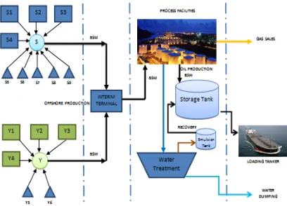
5737 fields and Y1-Y4 fields on Y field. There is also a STS type platform S5-S9 on S fields and Y5-Y6 fields in Y field. Both platform and STS operate close together and then flow accumulates towards one central platform. From the central platform oil and gas will be sent to the Onshore Terminal for further processing. Onshore Terminal consists of several plants (processing plants) which are used to process crude oil. Processed crude oil then sent by tanker for export commodities and processed gas for refineries.
Figure 2.1 Schematic diagram for South Area PT MLG
Oil and natural gas has long been a major backdrop in the fulfillment of world energy needs. Since petroleum is the main backing of almost every country and every line of industry, government, housing and property, households need energy. This can be evidenced by the facts contained in the annual report of one of the world's largest oil and gas energy companies, BP Petroleum [3]. Petroleum is believed to originate from fossils that are transformed into hydrocarbons after thousands of years through the process of change and journey and finally trapped in a reservoir. Indonesia is one of the organic regions and the ring of a volcano that houses or traps oil and gas [4]. The lifting of petroleum and natural gas from inside the bowels of the earth is known as exploration and production. Exploration activities are begin with the discovery of oil and gas reserves to performing drilling activities. Production is the activity of exploitation of general operation of oil and gas field after completion of drilling activities [8].
There are several general theories as to how the oil and gas can be lifted up to the surface and then finally purified and processed. Generally known by three kinds of terms, there was natural flow, artificial lift and EOR.
2.1.1 Natural Flow
Natural flow is the process of lifting the oil and the earth from the reservoir or oil reserves naturally. Natural flow exists because the new well reserves usually have enough pressure to get out of the earth. The pressure will push the desired oil or gas onto the surface and controlled its flow rate through some high pressure surface equipment. While the type of natural flow type itself can be controlled over two kinds of control. Gas Drive if the power comes from gas pressure and Water Drive if the power used comes from water pressure [9].
2.1.2 Artificial Lift
It is referred to as the method of recovering the oil using aid and artificial pressure. This method is required if reservoir pressure solely can not push the oil to rise up to the surface. Usually not enough gas and water pressure as it is in the natural flow wells. In contrast to the natural well type of flow, the artificial lifts are usually between 10 and 30 years old. The methods used for artificial lifts vary greatly among others. Gas lift, is a method of inserting gas into a well pipe intended for a reservoir that currently has little pressure but is unable to lift the oil to the surface. The purpose of gas lift is to reduce the density of the oil so the oil will lifted to the surface. Electric Submergible Pump which known as ESP, is a method of inserting a pumping body into a well tube at a depth of 300 to 1500 meters of underground. The purpose of ESP is to pump oil to reach the surface. Sucker Rod is a method of removal of oil using a nod pump. The self-propelled pump is driven by a motor on the surface.
2.1.3 Enhanced Oil Recovery
5738
2.2 Standard of Crude Oil Sampling
Crude oil analysis results from pipelines sampled correctly will indicate the quality and operating conditions of the existing process. So it can be used as a quality control of crude oil into storage tanks. Appropriate measurement using two methods. World general standards of sampling methods are embodied in ASTM D4057 (American Petroleum Institute) [2].
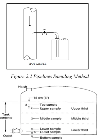
1. The sampling method of the process pipeline is illustrated in Figure 2.2 in which the sample is drawn from the stream inside the pipe through a small pipe.
[image:4.612.97.290.302.581.2]2. Composite sampling method as illustrated in Figure 2.3, composite is defined as a mixture of 3 sample types from three upper, middle and bottom taking points.
Figure 2.2 Pipelines Sampling Method
Figure 2.3 Storage tank composite sampling method
2.3 Stakeholder Parties
South Area operates certainly not stand alone and will affect each other in the operation. In addition to mutual influence and interrelated, the stakeholders also require the accuracy of production data produced by the production team. The stakeholders involved directly are as follows:
2.3.1 TS Lab (Team Support Laboratory)
TS Lab is the most relevant internal department and works closely with the operation, where almost all products produced by the operation are periodically controlled by this department. Crude oil samples include Incoming and Outgoing crude oil, separator outlet and inlet storage tank taken every 4 hours for BSW and API analysis.
2.3.2 Team Asset
Team assets are the team that manages and analyzes, then calculates and decides all the things about good governance. The asset team monitors the reserves and operation of the production well. Each well intervention activity then the asset team should pay attention to the risks and effects to the operation, in the sense that the interfence performed will provide a new product specification that gives the impact of the process to adapt again.
2.3.3 Operation specialist
There are departments that assist the operation in terms of analysis and daily process operations. Just as the asset team that interfacial activity on the process will affect the quality of production in the terminal. If the asset team focuses on upstream business then the specialist operations team focuses on downstream operations.
2.3.4 PAGO - Production Avails and Gas Operation
The PAGO team is a stakeholder operation in the field of data validity, they work as the final gateway of total gas and petroleum production. In addition, all data related to quality also boils down to PAGO, such as waste water data and air quality monitoring. The way it works is the system, therefore if there are input errors it will affect incorrect allocation data as well. The PAGO team is a team that represents operations when presenting data in management and to other customers outside the company. If there is any incompatibility of the data against the specification then the PAGO team will notify the operation team.
2.4 Definition of Artificial Neural Network
5739 through the network. Because of its adaptive nature, ANN is also often called the adaptive network [10].
Simply put, ANN is a non-linear statistical data modeling tool. ANN can be used to model the complex relationship between input and output to find patterns in the data. According to a theorem called "universal assessment theorem," ANN with at least a hidden layer with non-linear activation functions can model all of the Boreal's measured functions from one dimension to another.
The human brain (also animal) consists of cells called neurons. Compared to other cells that always reproduce themselves and then die, neurons have the privilege of not dying. This causes the information stored in it to survive. It is estimated that the human brain consists of 109 neurons, and
there are 100 known types of neurons. These neurons are divided into groups (called tissues) that are differentiated by function and each group contains thousands of interconnected neurons. Thus it can be concluded that the brain is a collection of neuronal tissues.
The speed of each network process is actually much smaller than the speed of the existing computer process at this time. But because the brain is made up of millions of networks that work in parallel (simultaneous), the brain can do a much more complex job than what a computer can do solely on speed. This parallel processing structure is another interesting part of the neural network, which can also be replicated to be implemented on a computer.
[image:5.612.314.529.39.242.2]Each neuron can have multiple inputs and one output. The input paths on a neuron may contain raw data or processed data on previous neurons. While the output of a neutron can be either the end result or an input material for the next neutron. An artificial neuron network consists of a collection of neuron groups arranged in layers. Inside ANN there is a modeling using multi layer perceptron type (MLP) with two hidden layers. The mathematical model for calculating output in the Multi Layer Perceptron (MLP) model or also known as Feedforward Neural Networks (FFNN) [11]. A simple configuration of the ANN algorithm can be explained in Figure 2.4:
Figure 2.4 ANN configuration
Input Layer (Input Layer)
The input layer serves as a link to artificial neural network or the Artificial Neural Network to the outside world (data source), each input will be determined its weight before being processed in the system.
Hidden Layer
A network can have more than one hidden layer (hidden layer) or even can not have it at all. If the network has several hidden layers, then the bottom hidden layer serves to receive input from the input layer.
Output Layer (Output Layer)
The working principle of neurons in this layer is similar to the working principle of the neurons in the hidden layer and here also the Sigmoid function is used, but the output of the neurons in this layer is considered to be the result of the process.
3. METHODOLOGY
Data structures in the study, among others, are described as in table 3.1 which includes t as the day of the day order of data collected and used.
Table 3.1 Data Structure
t St BSWSt Yt BSWYt Zt Ot
1 2 3 4 5 .
n
S1
S2
S3
S4
S5
. Sn
BSWS1
BSWS2
BSWS3
BSWS4
BSWS5 .
BSWSn
Y1
Y2
Y3
Y4
Y5
. Yn
BSWY1
BSWY2
BSWY3
BSWY4
BSWY5 .
BSWYn
Z1
Z2
Z3
Z4
Z5
. Zn
O1
O2
O3
O4
O5
. On
Where:
[image:5.612.311.514.570.713.2]5740 St : Daily Gross Production at Location S
Offshore
BSWSt : Daily Base Sediment and Water Location
S Offshore
Yt : Daily Gross Production at Location Y
Offshore
BSWYt : Daily Base Sediment and Water Location
Y Offshore
Zt : Net Offshore Production (Offshore Field)
Ot : Crude Oil Net Production (Onshore)
The data continued with St and Yt are the
gross fluid streams that still contain water and sediments in each of the S and Y fields, whereas BSWSt and BSWYt are water and sediments in each
St and Yt. Zt is the data generated from the
multiplication equation {S, Y, BSWSt, BSWYt}
which will be explained next, and Ot is the daily
net production of the Onshore.
3.1 Classic Assumption Tests
Regression test using OLS method requires Best Linear Unbiased Estimator (BLUE) from the estimator [6]. A series of tests can be performed so that the regression equation formed can meet BLUE requirements, namely normality test, multicollinearity symptom test, and autocorrelation symptom test.
3.1.1 Normality test
The normality test aims to test whether in the regression model the outlier or residual variable has a normal distribution. The normality test is important because the t-test and the F-test assume that the residual value should have a normal distribution value [6]. Normality tests were performed on the unstandardized residual values of the regression model using the One Sample Kolmogorov-Smirnov Test. Data are categorized as normal distribution if they produce asymptotic significance value> α = 5%.
Table 3.2 Autocorrelation testing Durbin-Watson (DW)
Hypothesis Zero Decision If There is no positive
autocorrelation There is no positive
autocorrelation No negative
correlation No negative
correlation There is no
autocorrelation, positive or negative
Decline
No decision Decline
No decision Not rejected
0 < d < dl
dl < d < du
4 - dl < d < 4
4 - du < d < 4 - dl
du < d < 4-du
3.1.2 Multicolinearity Testing
Multicollinearity test aims to test whether the regression model found a correlation between independent variables (independent). The method used to detect the presence of multicollinearity in this study by using the value of Variance Inflation Factor (VIF). A common cut-off value is used to indicate the presence of multicollinearity if the value of VIF produced is greater than 10 [6].
3.1.3 Autocorrelation Testing
The autocorrelation test aims to test whether in the linear regression model there is a correlation between the confounding error in period t with error in period t-1 (previous). If there is correlation, then there is called autocorrelation problem. The presence or absence of autocorrelation can be detected using the Durbin Watson (DW-test) test.
Durbin Watson's test is only used for first order autocorrelation and requires an intercept (constant) in the regression model with no lag variable among independent variables. Testing autocorrelation with Durbin Watson method will result in the decision is rejected or not rejected as listed in table 3.2.
3.2 Model Development
The statistical test of the research was conducted using two models, multiple linear regression test using Ordinary Least Squares (OLS) and Neural Network (NN). NN is used to explain the randomly variable relationship of responses to its predictors so as to predict the problem of future and future production of Onshore production. With advanced testing using NN will be missed which model has better prediction ability, classical statistical model (linear regression) or machine learning (NN) model. The main statistical test equipment still uses linear regression test. The use of Neural Network (NN) model is done only to strengthen the conclusion that the regression model used can be a good predictor in explaining the relationship pattern among variables.
3.2.1 Multiple linear regression test
The test is carried out in two stages, by including the BSW variable of location S and Y on the second model (sensitivity test). By entering the BSW variable, it is known that the sensitivity level in predicting the change of value of Onshore (Ôt)
5741 validation. The test is done by pooled data at α = 5% with equation as follows:
Ôt = β0 + β1St + β2Yt + β3Zt
Ôt = β0 + β1St + β2Yt + β3BSWSt + β4BSWYt
Where:
Ôt : Crude Oil Net Production (Onshore)
Βi : constants (n = 0,1,2,3)
St : Daily Gross Production at Location S
Offshore
Yt : Daily Gross Production at Location Y
Offshore
Zt : Net Offshore Production (Offshore Field)
BSWSt : Daily Base Sediment and Water Location
S Offshore
BSWYt : Daily Base Sediment and Water Location
Y Offshore
Testing is done partially to each independent variable. The rules of decision-making are:
- Probability (p) | t-test | <α, partially independent variables affect the dependent variable
- Probability (p) | t-test |> α, partially independent variable has no effect on dependent variable
3.2.2 Neural Network (NN)
ANN used in this system uses the type of Multi Layer Perceptron (MLP) with two hidden layers. This form of neural networks architecture (NN) is the most common and most widely used model in engineering or engineering applications. This model is also known as Artificial Neural Networks (FFNN) [11].
3.2.3 Model Comparison
With further testing will be found which model has better prediction ability, classical statistical model (linear regression) or machine learning (NN) model. Comparative model is done by comparing the Root Mean Square Error RMSE value. The smaller the resulting RMSE indicates that the model is getting better at predicting the value of the dependent variable.
4. RESULTANDDISCUSSION
Descriptive analysis is done by first doing the separation of data. Then will be presented characteristics of data consisting of the mean (mean), minimum, maximum, and standard deviation. The statistical test was performed using two models, multiple linear regression using Ordinary Least Square (OLS) and Neural Network (NN). Testing using Neural Network (NN) is done to reinforce the results of conclusion that the regression model used can be a good predictor in
explaining patterns of relationships between variables.
4.1 Results Of Regression Tests
4.1.1 Windowing 60 Days
Tests performed on the last 60 days data from pooled observation data on November 2, 2016 until December 31, 2016. The simultaneous test results in Table 4.1 for model I yielded F-test of 21,800 with significance (p) of 0%, the value of determination coefficient (R2) is 53.9%. This result
shows that during the 60-day observation period the model has been able to predict the variation of the change in onshore production value (Ôt) quite well
with the RMSE value is 746.452.
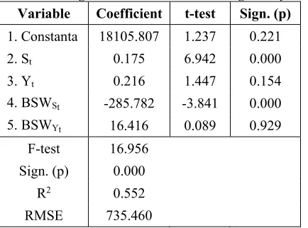
With the same treatment on model I simultaneous test results in Table 4.2 yielded F-test of 16.956 with significance (p) of 0%, the value of determination coefficient (R2) is 55.2%. These
results indicate that in the 60-day observation period the model has been able to predict the variation of the onshore (Ôt) production value
[image:7.612.314.522.398.543.2]changes quite well with the RMSE value being 735.460.
Table 4.1 Regression Model I windowing 60 days
Variable Coefficient t-test Sign. (p)
1. Constanta -6586.725 -1.735 0.088
2. St 0.070 2.027 0.047
3. Yt 0.239 1.979 0.053
4. Zt 0.561 3.600 0.001
F-test 21.800 Sign. (p) 0.000
R2 0.539
RMSE 746.452
Table 4.2 Regression Model II windowing 60 days
Variable Coefficient t-test Sign. (p)
1. Constanta 18105.807 1.237 0.221
2. St 0.175 6.942 0.000
3. Yt 0.216 1.447 0.154
4. BSWSt -285.782 -3.841 0.000
5. BSWYt 16.416 0.089 0.929
F-test 16.956 Sign. (p) 0.000
R2 0.552
[image:7.612.312.529.565.726.2]5742
4.1.2 Best Formed Regression Model
From the table summaries 4.1 and 4.2 it is found that the best regression model to predict the variation of the change of production value onshore (Ôt) is during the period of windowing 60 days
using the second model where the second stage testing included BSWSt and BSWYt variables
represented by BSW factor. The regression model that formed can be described as follows:
Ôt = 18105.807 + 0.175St + 0.216Yt – 285.782
BSWSt + 16.416 BSWYt
Based on the regression model above, the regression coefficient of St obtained by 0.175. This
result indicates that if variable of St rose by 1 unit
with assumption of other independent variable fixed value, will be followed by increase of Ôt
equal to 0.175 unit. The regression coefficient Yt is
0.216. This result indicates if the Yt variable goes
up by 1 unit with the assumption that the other independent variable is fixed, followed by the increase of Ôt of 0.216 unit. BSWSt regression
coefficient was obtained at -285.782. These results indicate if the BSWSt variable rises by 1 unit with
the assumption that the other independent variable is fixed, will be followed by a decrease of Ôt of
285.782 units. BSWYt regression coefficient was
obtained for 16.416. These results indicate that if the BSWYt variable rises by 1 unit with the
assumption that the other independent variable is fixed, it will be followed by a rise of Ôt of 16.416
units.
4.2 Test Results Of Neural Network (NN)
The neural network architecture that will be created is 3 layer feed forward network. The 3 layer network neural feed forward network consists of input layer, hidden layer, and output layer. The data used in the training are daily data of offshore oil production and BSW percentage. The experimental stage is done with the following series:
1. Determining the number of neurons in the hidden layer. The number of neurons used in each observation period is determined starting from a number of 1 neurons and limited to 25 neurons. 2. Determine the activation function to be used. The activation function uses two functions of Sigmoid Logistic and Tanh (Hyperbolic Tangent).
3. Determine the preprocessing method to be used. The preprocessing method uses 3 Standardized, Normalized and Adjusted Normalized methods.
4. Running program on SPSS version.23. Total running combination is done as much as 300 times obtained from: 2 model ൈ 25 hidden layer ൈ 2 activation function ൈ 3 preprocessing method. 5. Calculate the RSME value of each combination of errors obtained on the actual Ot difference with
Ôt prediction.
6. Choose the best model based on the smallest RMSE value.
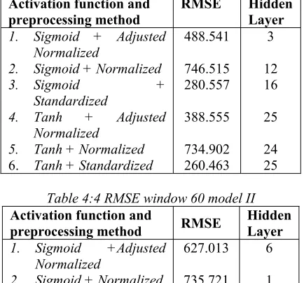
And the experiment give the best results based on Table 4:3 and 4:4 it is found that the development of the best ANN model to predict the variation of the change of production value onshore (Ôt) is during the period of windowing 60 days with
the number of neurons in hidden layer 8 using model II and activation function of Tanh (Hyperbolic Tangent) and Standardized preprocessing method with RMSE 208,919.
Table 4:3 RMSE window 60 model I Activation function and
preprocessing method
RMSE Hidden
Layer
1. Sigmoid + Adjusted
Normalized
2. Sigmoid + Normalized
3. Sigmoid +
Standardized
4. Tanh + Adjusted
Normalized
5. Tanh + Normalized
6. Tanh + Standardized
488.541
746.515 280.557
388.555
734.902 260.463
3
12 16
25
[image:8.612.310.527.346.548.2]24 25
Table 4:4 RMSE window 60 model II Activation function and
preprocessing method RMSE Hidden Layer
1. Sigmoid +Adjusted
Normalized
2. Sigmoid + Normalized
3. Sigmoid +
Standardized
4. Tanh + Adjusted
Normalized
5. Tanh + Normalized
6. Tanh + Standardized
627.013
735.721 334.395
418.357
718.891 208.919
6
1 9
21
5743
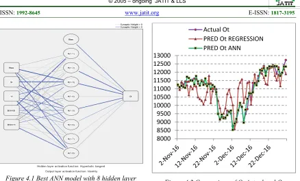
Figure 4.1 Best ANN model with 8 hidden layer 4.3 Result Discussion
From result of regression test and model development using artificial neural network each found the best model. The best regression test yielded RMSE 735.460 and model development using ANN resulted in a model with smaller RMSE 208.919. It has been seen that the model generated by the development through ANN produces better results marked with much smaller RMSE value, meaning that the prediction of ANN model to Ôt
value is much more accurate. Figure about Neural Network architecture showed in Figure 4.1. Then there is showed the actual Ot visualization by Ôt
prediction of regression and ANN through figure 4.2.
Figure 4.2 Comparison of Ot Actual and Ot
Prediction Charts
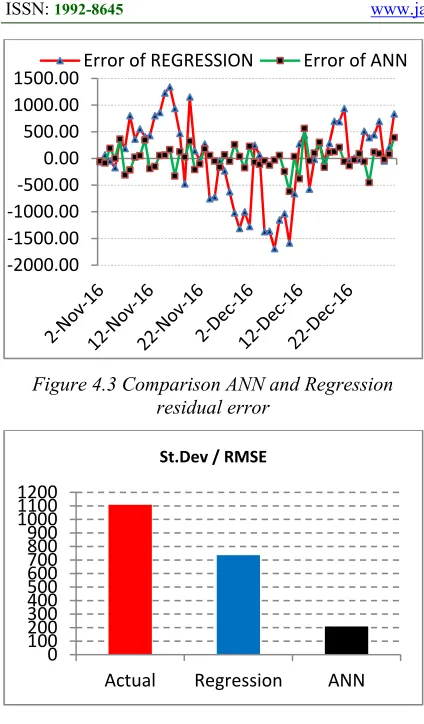
To further support the comparison and determination of the best model it is necessary to add an advanced analysis. Then presented a graphical visualization of how the model generated by ANN is very coincident with the daily production value of Ot onshore. Therefore the
following error values are generated by each of the best regression prediction models and the best ANN in Table 4.28 and Figure 4.3. The comparison between the standard deviation or the RMSE on the actual Ot and Ot predictions of each regression as
well as ANN is depicted in Figure 4.4.
BSW on model II here proved to be more influencing predictive model compared to Zt on
model I which is the daily production of offshore net itself. Therefore, in order to maximize the results of the model in order to get RMSE hope that is smaller then BSW measurement method should be more precise. The daily average withdrawal method has a larger error rate and is less representative of the actual daily BSW. In some modern locations have applied a method of measurement continue by using electromagnetic radiation, which at any time the tool will provide recording and reporting online into the desired system.
8000 8500 9000 9500 10000 10500 11000 11500 12000 12500 13000
Actual Ot
5744
Figure 4.3 Comparison ANN and Regression residual error
Figure 4.4 Comparison Actual St.Dev and RMSE of Model
Measurement method which has also been applied at other location is with automatic sampler in piping system. Automatic sampler has actually been applied to PT MLG but still limited to custody transfer of petroleum sales. How this automatic sampler works is the presence of a motor that drives a small pump on a stroke that has been setting and regularly take oil from the pipeline with a very small dose. The small dosage setting can be changed to aim for a specified amount of petroleum sampling and the time specified.
Since BSW is measured to be a factor affecting daily net forecasts of onshore petroleum models, it should also be considered that temperature variables can be part of a model prediction. This can be considered for the development of the next model to allow for more accurate and varied models to predict daily onshore production. Such temperatures can be obtained from daily readings of outgoing petroleum lines at measured offshore locations with Zt.
V. CONCLUSIONANDRECOMMENDATION
5.1 Conclusion
Based on the results of the analysis in the previous chapter, some conclusions can be drawn from the research are as follows:
1. Regression test results using Model II full observation year showed that BSW of both sites had a significant negative effect on the onshore ground production (Ôt). These results indicate
that the higher the BSW content will be followed by a significant decrease in onshore production (Ôt). The best regression model
formed can be described as follows:
Ôt = 18105.807 + 0.175St + 0.216Yt – 285.782
BSWSt + 16.416 BSWYt
Based on the regression model obtained RMSE value 735.460.
2. The best ANN model to predict the variation of the change of production value onshore (Ôt) is
during the period of windowing 60 days with the number of neurons in the hidden layer 8 using the model II using the variable St, Yt,
BSWSt and BSWYt as well as activation function
Tanh (Hyperbolic Tangent ) And Standardized preprocessing methods. Based on this artificial neural network model obtained RMSE value 208.919.
3. Based on comparison of best regression model with RMSE 735.460 value compared to best ANN model with RMSE value 208.919 then ANN Model is the best model in explaining relationship pattern between offshore production and onshore production area south of PT MLG.
B. Recommendation
Some suggestions that can be given based on the results of research are:
1. For further research, research can be developed by using window period around data indicated is a 60 day outlier. With the development is expected to obtain a more complete analysis results when associated with the possibility of the pattern of intervention in the well and reservoir. The use of other broader statistical testing tools such as the use of structural equation modeling, deserves consideration. 2. For further research, research can be developed
by using temperature measurement variable. Measurement temperatures can be obtained from temperatures in offshore pipes or from
‐2000.00 ‐1500.00 ‐1000.00 ‐500.00 0.00 500.00 1000.00
1500.00Error of REGRESSION Error of ANN
0 100 200 300 400 500 600 700 800 900 1000 1100 1200
Actual Regression ANN
5745 measurements obtained in onshore tanks. Temperature as disclosed in this paper as a determinant factor for the net volume of petroleum.
3. For policymakers in PT MLG, it is expected to consider increasing the frequency of BSW taking. Currently BSW offshore taking mechanism is performed 6 times during the day, and from the taking in the average to get one value to be used as the basis for determining offshore production. High differences could be due to the inaccurate and fluctuating BSW values, as indicated by the sensitivity analysis that BSW has an effect on offshore production. 4. For policymakers in PT MLG, it is desirable to
consider applying a continuous measurement method using modern BSW measurement tools using electromagnetic radiation equipment such as x-rays and the like, which at any time will provide recording and reporting online to the system. Also worth considering the method of measurement that has also been applied at other locations is with automatic sampler on the piping system.
REFERENCES:
[1] Aizenberg, I., Sheremetov, L., Vargas, L.V., and Martines, J.M. Multilayer Neural Network with Multi-Valued Neurons in time series forecasting of oil production. Neurocomputing vol. 175 (2015),pp 980-989.
[2] American Petroleum Institute. (2012). ASTM D4057, Manual of Petroleum Measurement Standart Chapter 8.1. Pennsylvania United States: ASTM International.
[3] British Petroleum. (2016). BP Statistical Review of World Energy. London, UK: Centre for Energy Economics Research and Policy Heriot-Watt University.
[4] Chevron Corporation. (2015). Annual Report Supplement. San Ramon, California, USA: Chevron Corporation.
[5] El-Abbassy, M., Senouci, A., Zayed, T., Mirahadi, F., and Laya P. Artificial neural network models for predicting condition of offshore oil and gas pipelines. Automation in Construction vol 45 (2014), pp 50-65.
[6] Gujarati, D. Basic Econometrics. (2006). Jakarta: Erlangga.
[7] Jakobsson, K., Soderbergh, B., Snowden, S., and Aleklett, K. Bottom-up modeling of oil production: A review of approaches. Energy Policy vol 64 (2013), pp 113-123.
[8] Ministry of Education and Culture.. (2013). Basic Drilling Technique. Jakarta: Directorate of Vocational Secondary Education.
[9] Ministry of Education and Culture.. (2013). Reservoir Engineering and Oil and Gas Reserves. Jakarta: Directorate of Vocational Secondary Education..
[10]Specht, D. F. (1991). A General Regression Neural Network. Neural Network, Volume 6 Issue 7, 568-576.
[11]Suhartono. (2007). Feedforward Neural Network For Time Series Modeling, Dissertation Department of Mathematics, Yogyakarta: Universitas Gajah Mada.
[12]Torsun, E., Aydin, K., dan Bilgili, M. Comparison of linier regression and artificial neural network model of a diesel engine fueled with biodiesel-alcohol mixtures. Alexandria Engineering Journal vol 55 (2016), pp 3081-3089.