An Efficient Load Balancing Algorithm for Energy Utilization in Wireless Sensor Network

An Efficient Load Balancing Algorithm for Energy

Utilization in Wireless Sensor Network

Rajendra S. Navale

SKNCOE, Pune

Vaishali S.Deshmukh

SKNCOE, Pune

ABSTRACT

In recent days Wireless Sensor Network has grown up very vastly. Energy efficiency is the most important consideration in WSN. Many algorithms were developed for the purpose of energy efficiency. In WSN there are number of sink nodes present and this sink nodes may have different loads and because of this they require different energy for transmission of data to a particular base stations. But while implementation of network this sink node has generally same capacity and same energy power associated with it. If some sink nodes are having fewer loads, then they utilize less energy associated with it and vice versa. Here load is nothing but the number of base stations handled by that particular sink node. Due to underutilization and overutilization of energy by all the sink nodes, it is necessary to have some technique or algorithms that balance the load among all the sink nodes in WSN. To balance the load among all the sink nodes there were many algorithms developed. One of which is called as load balancing for energy utilization algorithm which was totally depend on Smart Boundary Yao Gabriel Graph(SBYaoGG) algorithm. And in this paper a new load balancing algorithm is presented which is called as Efficient Load Balancing Algorithm for WSNs. And also results of this new algorithm are discussed in results section.

Keywords:

1.

INTRODUCTION

Topology Control is a technique which is used to increase network capacity and to reduce energy consumption in ad hoc and wireless sensor network. The goal of Topology Control protocol is to reduce the transmission power level used by network nodes, with the constraint of preserving some fundamental properties (typically connectivity) of the communication graph. Decreasing the nodes transmission power with respect to the maximum level potentially has two effects:1)reducing the nodes energy consumption, and 2) increasing the spatial reuse, with a positive overall effect on network capacity[1].Sensor nodes are small in size and communicate unrestrictedly over short distances. They have sensing, data processing and communication capabilities and their features have enabled, as well as provided, impetus to the idea of Wireless Sensor Networks (WSNs)[2]. WSNs are powerful and they support lot of real world applications. Networks of sensors exist in many industrial applications providing the ability to monitor and control the environment in real time .Most of the sensor networks are wired and because of this they are costly to install and maintain. To reduce the cost of installation and maintenance of wired sensor network a wireless sensor networks are developed. Other benefits of Wireless sensor networks are easy to deploy,

reduced danger of breaking the cables and less hazels with connectors, and easy to use, enhanced physical mobility.

A Sensor Network is composed of a large number of sensor nodes that are densely deploy either inside the phenomenon or very close to it[3]. The positions of the sensor nodes in the sensor network need not be engineered or predetermined. Because of this it allows the random deployment of nodes in the network. The most important and unique feature of sensor network is co-operative efforts of sensor nodes. These sensor nodes are fitted with onboard processor. Instead of sending the raw data to the nodes responsible for the fusion, they use their processing abilities to carry out simple computations and transmit only required and partially processed data. Because of all above features sensor networks have many applications such as, Health, Military, home, and industrial. With the recent advances in wireless sensor networks (WSNs), the realization of low-cost embedded industrial automation systems have become feasible [3]. In these systems, wireless tiny sensor nodes are installed on industrial equipment and monitor the parameters critical to each equipment’s efficiency based on a combination of measurements such as vibration, temperature, pressure, and power quality. These data are then wirelessly transmitted to a sink node that analyzes the data from each sensor. Any potential problems are notified to the plant personnel as an advanced warning system. This enables plant personnel to repair or replace equipment, before their efficiency drops or they fail entirely. In this way, catastrophic equipment failures and the associated repair and replacement costs can be prevented, while complying with strict environmental regulations [6].The collaborative nature of IWSNs brings several advantages over traditional wired industrial monitoring and control systems, including self-organization, rapid deployment, flexibility, and inherent intelligent-processing capability. In this regard, WSN plays a vital role in creating a highly reliable and self healing industrial system that rapidly responds to real-time events with appropriate actions[2],[5].

Usually, the sensor nodes are designed to report measured information to a data sink node. Among the most common scenarios for sensor networks are environmental monitoring tasks, for instance to warn of imminent natural disasters or for the purpose of biological or other scientific observations [12].

2.

RELATED WORK

2.1

Load Balancing Routing Algorithm for

Multi-Sinks in WSN’s

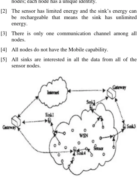
The system architecture of multi-sink wireless sensor networks which is considered for this algorithm is as shown in Fig 1. It has the following characteristics:

[1] The number of sensor nodes is larger than that of sink nodes; each node has a unique identity.

[2] The sensor has limited energy and the sink’s energy can be rechargeable that means the sink has unlimited energy.

[3] There is only one communication channel among all nodes.

[4] All nodes do not have the Mobile capability.

[5] All sinks are interested in all the data from all of the sensor nodes.

Fig 1: System Architecture of Multi-Sink WSN

And the steps for Multi-Sink Load-Balance Routing Algorithm are as follows:

Void PacketRouting(Packet P){

if (NodeID=P.DestID) {

//If the node is destination deputy node Transfersthe Packect to Sink.

}else{

RouteToNextHop(P,NodeID);

}

intRouteToNextHop(Packet P, intNodeID

intnexthop;

if(P.TimeToLive=0) return FALSE;// ro

DS1={dti1 | dti1 DS(NodeID), dti1.D

if(DS1 = Ø){

Randomly select a nti from DirtyLevelNT(NodeID);

nexthop =nti.NeighborID;

}else{

DS2 = {dti2 | dti2 DS1 /\ dti2.DirtyLevel

( dti1 DS1, FF(dti2.NextHpoIDP.DestID),

FF(dti1.NextHpoIDP.DestID)}

NT1 = {nti | nti NT(NodeID) /\ nti.DirtyLevel

nti.NeeghboeID DS2}

if(NT1 =Ø ){

Randomly select a nti from DirtyLevelNT(NodeID);

nexthop =nti.NeighborID;

}else{

Randomly select anti from NT1;

nexthop =nti.NeighborID;

}

nexthop =nti.NeighborID;

}

P.NextHoID = nexthop;//the nextis found

P.TimeToLive =P.TimeToLive – 1;

Transfer Packet P to P.NextHopID;

if(Transfer failed){//the next hop are not available;

update the DirtyLevel field in NT and DT;

RouteToNextHop(P, Ni)}else{return TRUE;}

}

}

2.2

Load Balancing for Energy Utilization

in WSN Algorithm

This algorithm is using to make topology in energy efficient state. Here in this algorithm first the energy load in each sink\state node is calculated. Then check the load of every sink node and if it has equal load then do nothing otherwise reduce the load from the sink nodes which are using high load and allocate this load to the sink nodes which are using less load. Here it was assumed that more load to a particular sink node means it requires more energy to handle that load and vice versa.

The Load balancing for energy utilization algorithm is given below:

1. The node discovers its neighbor nodes by broadcasting at maximum power.

2. Unit Disk Graph (UDG) is calculated by using Waxman Algorithm.

3. Apply SBYaoGG.

4. Check load on each sink node.

1. If each state node has equal load then do nothing.

Finally, results are shown to be work favorably and it gives good result.

This algorithm takes an output of SBYaoGG algorithm as input to it. The SBYaoGG algorithm was mainly developed for the purpose of energy efficiency and to lower the interference in the wireless sensor network. But the final graph of SBYaoGG contains some sink nodes having high load than others and vice versa. And for better utilization of energy in WSN it was necessary to balance the load among all the sink nodes so that energy utilization in network will be reduced.

2.2.1

Disadvantage

This algorithm only removes the load of overloaded sink nodes and assigns it to under loaded sink nodes without considering the distance of each base station from the each sink node. Because of this some time the base station which is far away from the sink node is allocated to it than the other base station which is close to that sink node. So because of this the distance for data transmission increases and consequently the energy required for that particular sink node is increased and it again utilizes the high energy.

To overcome with this disadvantage the new algorithm for load balancing is developed called as “Efficient Load Balancing Algorithm for Energy Utilization in WSN” and it is discussed in the next section.

3. EFFICIENT LOAD BALANCING

ALGORITHM (Proposed Algorithm)

This algorithm is the enhanced part of the Load Balancing for Energy Utilization in WSNs Algorithm discussed in previous section. To overcome with the disadvantage as stated in previous section, this new algorithm is proposed and it works favorably.

Here all the steps of algorithm are same as previous algorithm exception is that when extra load is allocated to particular sink node (sink node having less load than mean load) the care should be taken as the only base station which is near to that particular sink node is allocated to it. Because of this the distance travelled by data to reach at each destination will be reduced and consequently energy utilization by sink node is also gets reduced. This procedure is applicable for all the sink nodes so that all sink nodes are get balanced with base stations which are near to it.

The steps for Efficient Load Balancing Algorithm for energy utilization in wireless sensor network are as follows:

1. The node discovers its neighbor nodes by broadcasting at maximum power.

2. Unit Disk Graph (UDG) is calculated by using Waxman Algorithm.

3. Apply SBYaoGG algorithm.

4. Calculate the total load on all sink nodes by using the following formula-

Let TSL be the total of all load, then

TSL =

Where SL be the set of all state nodes load then

SL = { SL1, SL2, SL3, …, SLn }

5. Calculate the mean load that will be on every sink node by using the following formula-

MinLoad = TSL / n

Where n is the number of sink nodes in the network.

6. Check load of each sink node if it is equal to mean load then do nothing otherwise;

7. Remove the excess load from overloaded sink nodes and assign it to under loaded sink nodes subject to following conditions:

7.1 Allocate the base station which is near to under loaded sink node so that distance will be minimized and the distance between sink nodes and the base stations are calculated by using following formula:

Lx = (xPosition(p1) – Position(p2))2

Ly = (yPosition(p1) – Position(p2))2

L =

7.2 while balancing the load firstly calculate the number of sensor nodes which are coming under the particular base stations. Because of this while balancing the load it should be considered that how much sensor nodes are there in particular base stations. So after the load balancing all the sink nodes generally handles approximately same number of base stations and consequently approximately same number of sensor nodes.

4. RESULT

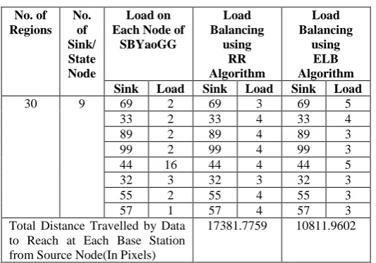
For discussion of results, here we have considered 100 numbers of sensor nodes and 30 region boundaries.

Table 1. Comparison Values

These results were taken by using .Net framework .So here after random calculation 9 sink nodes are coming within that network. And because of 30 regions there are 30 base stations i.e. one base station for each region. The above table shows the number of sink/state nodes and number of loads on that sinks for SBYaoGG algorithm, Round Robin algorithm and for Efficient Load Balancing algorithm. Also the distance travelled by data to reach at each base station from source node for round robin algorithm and efficient load balancing algorithm are shown. The distance requirement for ELB algorithm is less than the RR algorithm. Here less distance travelled means less energy utilization by sink nodes and consequently by whole network because every sink node will have to visit minimum distance so energy utilized by every No. of

Regions No.

of Sink/ State Node

Load on Each Node of

SBYaoGG

Load Balancing

using RR Algorithm

Load Balancing

using ELB Algorithm Sink Load Sink Load Sink Load

30 9 69 2 69 3 69 5

33 2 33 4 33 4

89 2 89 4 89 3

99 2 99 4 99 3

44 16 44 4 44 5

32 3 32 3 32 3

55 2 55 4 55 3

57 1 57 4 57 3

Total Distance Travelled by Data to Reach at Each Base Station from Source Node(In Pixels)

sink will also get reduced. And hence in this way it is possible to reduce the energy utilization by whole network.

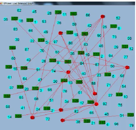
The results of these algorithms are shown below. Here UDG graph is not shown because there are different ways or algorithms on which UDG is calculated. it depends on you that how UDG should be created. Here in this algorithm UDG is created using Waxman algorithm. For above table 1 the SBYaoGG graph will look like as follows:

Fig 2: SBYaoGG

Fig 3: Round Robin

Round robin algorithm for load balancing in WSN when applied on that SBYaoGG then the final graph after load balancing will look like as shown in figure3. Here loads to particular sink nodes are get balanced. But the working of load balancing algorithm is taking long distance traversal for visiting every base station in network. It is because it first visits the sink node which is near to source node and then visits a base station which is near to that sink node then it moves to another sink node which is little longer than first sink node and visits it and again it visits to a base station which is near to that sink node and so on. After visiting every

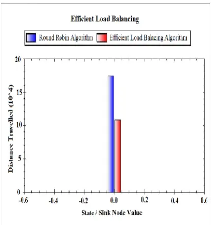
sink node it comes again to a first sink node and visits second near base station for that particular sink node and then moves to next sink node which is second near to source node. And then it visits to second nearest base station and so on. In this way to visit every base station from source node by using Round Robin algorithm requires 17381.7759[in pixels] or 459.8928[in centimeters] distance.

Fig 4: Efficient Load Balancing

Now when proposed algorithm is applied on SBYaoGG then its graph will look like as shown in figure 4. Here also loads are get balanced approximately same as by Round Robin Algorithm which is shown in figure 4. And for this algorithm total distance travelled by data to reach at each base station will be 10811.9602[in pixels] or 286.0664 [in centimeters]. So because of less distance required to transmit data at each destination the energy consumed by sink nodes will also be gets reduced.

Fig 5: Comparison of RR and ELB for loads on each Sink / State node

Fig 6: Comparison of ELB with RR by Distance Factor

5.

CONCLUSION

In this paper a load balancing algorithm for energy utilization in wireless sensor network was developed in the form of Efficient Load Balancing algorithm. Results of Efficient Load Balancing algorithm were compared with an existing Round robin algorithm and it works favorably. Also in this paper the graphs for SBYaoGG algorithm, Round Robin algorithm and Efficient Load Balancing algorithm are shown and from which the concept for new algorithm (ELB) was more cleared. In future this algorithm can be used for more region boundaries like 50, 70, 90 etc. This whole work was carried on .Net framework and Visual Studio 2010.

6.

REFERENCES

[1] Rajendra S. Navale, Vaishali S.Deshmukh”A Distributed Topology Control Technique for low interference and load balancing of energy utilization in WSNs.” International Journal of Engg. And Scientific Research, Vol.4, Issue7, Jully2013, ISSN2229-5518

[2] Tapiwa M. Chiwewe, student Member, IEEE, and Gerhard P. Hancke, Senior Member, IEEE “A Distributed topology Control Technique For Energy efficiency and Low Intereference In Wireless Sensor Networks” IEEE TRANSACTION ON INDUSTRIAL INFORMATICS,VOL.8, NO.1, FEBRUARY 2012.

[3] I.F. Akyildiz, W.Su, Y.Sankarasubramaniam, and E. Cayirci,” A Survey on sensor networks,” IEEE Commun. Mag.,vol. 40, no.8, pp.102-110, 2002.

[4] M.M. Shalaby, M.A. Abdelmoneum, and K. Saitou,” Design of spring coupling for high-Q high-frequency MEMS filters for wireless applications,”IEEE Trans. Ind. Electron., vol. 56, no. 4, pp. 1022-1030, Apr.2009.

[5] A.Willing,”Recent and emerging topics in wireless industrial communications: A selection,” IEEE Trans. Ind.Inform.,vol.4, no.2, pp.102-122, May2008.

[6] V.C.Gungor and G.P.Hancke,” Industrial wireless sensor networks: challenges, design principles, and technical approaches,” IEEE Trans.Ind.Electron., vol.56,no.10,pp.4258-4265, Oct. 2009.

[7] Alice Le Gall, Valerie Cialetti, Jean-Jacques Berthelier, Alain Reineix, Christophe Guiffaut, Richard Ney, Francois Dolon, and Sebastien Bonaime “An Imaging HF GPR Using Stationary Antennas: Experimental Validation over the Antartic Ice Sheet,” IEEE TRANSCATION ON GEOSCIENCE AND REMOTE SENSING, VOL.46, NO.12 DECEMBER 2008.

[8] V.C gungor, B. Lu, andG.P. Hancke,” Opportunities and challenges of wireless sensor networks in smart grid,” IEEE TRANS. Ind. Electron., vol.57, no.10,pp.3557-3564, Oct.2010.

[9] A. Koubaa, R. Severnio, M. Alves, and E. Tovar,” improving quality of service in wireless sensor network by mitigating hidden-node collisions,” IEEE Trans. Ind.Inform., vol.5, no.3, pp.299-313, Aug.2009.

[10] D.M. Blough, M.Leoncini, G.Resta, and p. santi”The K-Neigh protocol for symmetric topology control in ad hoc networking and computing, 2003, pp.141-152.

[11] P.von Rickenbach, R. Wattenhofer, and A. Zollinger,” Algorithmic models of interference in wireless ad hoc

and sensor networks,”IEEE/ACM

Trans.Networking.vol.17, no. 1,pp. 172-185, Feb.2009.

[12] L.Li, J.Y.Halpern, P.Bahl, Y-M.Wang,and R.Wattenhofer,”a cone based distributed topology control algorithm for wireless multi hop networks,” IEEE/ACM Trans. Networking,vol.13, no.1.pp.147-159,Feb.2005.

[13] P. santi and D.M. Blough,” The critical transmitting range for connectivity in sparse wireless ad hoc networks,” IEEE Trans. Mobile Computing,vol.2, no. 1, pp.25-39, Jan-Mar.2003.

[14] V.Kawadia and P. R. Kumar,”Principles and protocols for power control in wireless ad hoc networks,” IEEE J.Sel. Areas Commun, vol.23, no. 1, pp.76-88, Jan.2005.

[15] A. Cerpa and D. Estrin,” ASCENT: Adaptive self configuring sensor networks topologies”, IEEE Trans. Mobile Comput, vol.3, pp.272-285, Jul-Aug.2004.

[16] Piotr Zwierzykowski, Maciej Piechowiak “ The Influence of Network Topology on the Efficiency of Multicst Heuristic Algorithms”.