Munich Personal RePEc Archive
Estimating a preference-based single
index from the Asthma Quality of Life
Questionnaire (AQLQ)
Yang, Y and Tsuchiya, A and Brazier, J and Young, Tracey
A.
2007
Online at
https://mpra.ub.uni-muenchen.de/29804/
HEDS Discussion Paper 07/02
Disclaimer:
This is a Discussion Paper produced and published by the Health Economics
and Decision Science (HEDS) Section at the School of Health and Related
Research (ScHARR), University of Sheffield. HEDS Discussion Papers are
intended to provide information and encourage discussion on a topic in
advance of formal publication. They represent only the views of the authors,
and do not necessarily reflect the views or approval of the sponsors.
White Rose Repository URL for this paper:
http://eprints.whiterose.ac.uk/10917/
Once a version of Discussion Paper content is published in a peer-reviewed
journal, this typically supersedes the Discussion Paper and readers are invited
to cite the published version in preference to the original version.
Published paper
None.
H
H
e
e
a
a
l
l
t
t
h
h
E
E
c
c
o
o
n
n
o
o
m
m
i
i
c
c
s
s
a
a
n
n
d
d
D
D
e
e
c
c
i
i
s
s
i
i
o
o
n
n
S
S
c
c
i
i
e
e
n
n
c
c
e
e
D
D
i
i
s
s
c
c
u
u
s
s
s
s
i
i
o
o
n
n
P
P
a
a
p
p
e
e
r
r
S
S
e
e
r
r
i
i
e
e
s
s
No. 07/02
Estimating a pr efer ence-based single
index fr om the Asthma Quality of Life
Questionnair e (AQLQ)
Yaling Yang, Aki Tsuchiya, John E. Brazier, Tracey A. Young
Corresponding author: Yaling Yang ([email protected])
HEDS, ScHARR, University of Sheffield
Regent Court, 30 Regent Street, Sheffield, UK, S1 4DA
Tel: +44 (0) 114 2226386
Abstr act: This paper presents a study to estimate a preference-based single index from the Asthma Quality of Life Questionnaire (AQLQ). Based on the AQL-5D which is a health classification system directly derived from AQLQ, 98 health states was valued by a sample of 307 members of the UK general population. Models were estimated to predict all possible 3125 health states defined by the AQL-5D and compared using a set of criteria. The mean model of main effects was recommended of preferable prediction ability and logically consistent and significant coefficients for levels of dimensions. However, there are concerns over condition-specific valuation issues, such as presenting asthma
information to general public and the choice of condition specific full health as the upper anchor for TTO valuation.
Key words: AQL-5D, health state valuation, condition-specific, Time-trade-off, asthma
Acknowledgements
Intr oduction
Cost-effectiveness analysis has been widely used as a tool to support decision making on
health resource allocation in the last decade, especially with establishment of government
agencies such as the National Institute for Health and Clinical Excellence (NICE) in the UK
and similar agencies around the world (ISPOR, 2006). A cost-effectiveness study may
employ Quality Adjusted Life Years (QALYs) as the outcome measure to enable direct
comparisons across different health interventions or different medical conditions.
The QALY combines quality of life (expressed in terms of a “utility” score) and length of
life (in years) into a single index. The utility score reflects the quality of life of a given
health state and is elicited through valuation exercises, such as the Standard Gamble, Time
Trade-off (TTO), or the Visual Analogue Scale (VAS). The scores lie on a scale of 0 to 1,
where 0 is equivalent to dead and 1 equivalent to perfect health. Economic evaluations of
health care technologies can either carry out their own valuation studies of the health states
relevant to the given research project, or they can use “off the shelf” generic
preference-based instruments. These instruments have pre-scored health classification system and are
able to estimate utility scores for all possible health states: examples include EQ-5D (Dolan,
1997), Health Utility Index (HUI; Feeny et al, 2002), Quality of Well-being Scale (QWB;
Anderson et al, 1989) and SF-6D (Brazier et al, 2002). Such “off the shelf instruments”
have been widely used in cost-effectiveness studies not only because of their convenience,
A clinical trial often includes disease-specific quality of life instruments to capture clinical
efficacy, and increasingly, one of the generic preference-based instruments in order to
derive QALYs and to calculate cost effectiveness. Generic preference-based instruments
typically cover dimensions of health such as mobility, pain, activity limitation, and anxiety
or depression. However, for certain medical conditions, the set of dimensions covered by
generic measures may not be relevant, or even where relevant, they have been found to
insensitive (Guyatt GH, et al, 1999; Jenkinson C, et al, 1997) by missing ‘small but
important changes’ or requiring a larger sample size for some specific medical conditions.
At the same time, many clinical trials currently exclude generic measures, either due to
concerns about patient burden or because they are not regarded as appropriate by those
designing the trial. This disadvantage evoked the debate on roles of generic and
condition-specific health related measures in health care decision making, (Dowie J, 2002; Feeny D,
2002; Guyatt G; Brazier J, 2002).
One way to improve the sensitivity of generic preference-based measures is to broaden
their coverage to include dimensions relevant to the condition being considered (a condition
specific ‘add-on’). While this approach is worth exploring, another approach is to obtain
preference weights for a condition specific descriptive system. This has the advantage that
it ensures that the health state utility scores used in economic evaluation better reflect the
impact of the medical condition; and secondly it makes better use of the condition-specific
measures where generic ones have been excluded. Several studies have been undertaken to
obtain health state utility values for condition-specific instruments, such as the
Utility Index (ASUI) (Revicki et al, 1998), the International Index of Erectile Function
(Stolk et al, 2003), health states related to erectile dysfunction (Torrance et al, 2004) and
Urinary Incontinence (Brazier et al, 2005).
There has been little written on the methods for developing a preference-based measure
from a condition specific measure. The study reported in this paper was undertaken to
develop a preference-based single index from an asthma-specific instrument.
The Asthma Quality of Life Questionnaire (AQLQ) has been designed to assess health
related quality of life in patients with asthma (Juniper et al, 1993; also see Juniper et al,
1999). It has been used in more than 170 papers quoted by Medline. However, the AQLQ
cannot be directly used in economic evaluation in its current form because it does not
incorporate preference information.
To derive a preference-based single index measure from the AQLQ, we used a
methodology successfully used on the SF-36 by Brazier et al (2002) to generate the SF-6D.
The first stage is to derive a reduced health state classification system from the AQLQ that
is amenable to valuation exercises using a preference elicitation technique. The second
stage is a valuation survey of a selection of states defined by this reduced classification
system, by a sample of the UK general population. The third stage is to estimate a range of
econometric models for predicting the health state values for all states defined by the new
classification system, which in turn will enable the calculation of health state utility values
This paper concentrates on the valuation survey and the econometric modelling. For the
derivation of the reduced classification system, see Young et al (2005).
The next section describes the AQLQ in more detail. This is followed by a brief description
of the reduced classification system used in the valuation survey. Section 3 describes the
methods involving in the valuation survey and modelling. Section 4 presents the results of
the study including the survey and the models. The final section discusses the results and
then use of condition specific preference-based measures in informing resource allocation
1. The AQLQ and the r educed classifica tion system
The AQLQ consists of 32 items with 7 levels each, covering 4 dimensions: symptoms (12
items), activity limitations (11 items), emotional function (5 items) and environmental
stimuli (4 items). Table 1 shows the 32 items in the AQLQ.
The original AQLQ is too large to be amenable to valuation. Therefore, based on the
application of Rasch analysis and conventional psychometric tests, the AQLQ has been
reduced to a 5- dimension health state classification system which we call AQL-5D (see
Table 2). The dimensions are: concern about asthma, shortness of breath, weather and
pollution stimuli, sleep impact and activity limitations. These dimensions are selected
directly from the original AQLQ. Each dimension has 5 levels of severity with level 1
denoting no problem and level 5 indicating extreme problem. All AQLQ health states
2. Methods
2.1 Valuation survey
The aim of the valuation survey is to elicit preference values from the general public for a
sample of health states defined by the AQL-5D. The key methodological issues are the
selection of health state sample to be valued, sampling of respondents and overall size of
the sample, effective way of presenting asthma disease information to general public, and
the technique for eliciting preferences.
2.1.1 Selection of health states
The selection of health states was determined by the specification of the model to be
estimated. In this study, 98 health states were selected out of the 3125 possible health states
defined by the classification. The selection was on the basis of a balanced design, which
ensured that any dimension-level (level of dimension ) had an equal chance of being
combined with all levels of the other dimensions. These 98 states were stratified into
severity groups based on their total level score across the dimensions (simply the sum of
the levels), and then randomly allocated into 14 blocks, so that each block has 7 health
states. This procedure ensured that each respondent, who were allocated one of the 14
blocks, received a set of states balanced in terms of severity and that each state is valued the
same number of times apart from the worst possible state, or the ‘pits’ state, which is
2.1.2. Respondents
An important methodological issue is whether to sample a group of patients or use a sample
of the general population (Drummond et al, 1997). However, health policy bodies such as
NICE have recommended using general public values. It was decided to elicit the
preference values of general public although this instrument is a condition specific
questionnaire.
The respondents are members of the general population randomly selected using the
electoral register of names and address from within South Yorkshire, UK. Based on previous experience, we decided to interview a sample of 300 participants providing
valuations for 98 health states, which were deemed sufficient to estimate a reliable additive
model.
2.1.3 Pilot study on pr esentation of asthma infor mation
Given that it might be a problem for members of the general public to imagine what it is
like to live with asthma, two different ways in which to present information on asthma were
piloted on 100 respondents selected in the same way though not included in the main
survey. The first presentation was based on around 180 words of verbal information printed
on a card (taken from the British Thoracic Society website, see Appendix 1), and the other
was based on two brief video clips (provided by Asthma UK, and Wellington Asthma
Research) showing the biological mechanism of asthma and patients with asthma
Interviews were undertaken in the same way as in the main valuation survey (see 2.1.5)
with one “block” containing eight health states. In order to choose one block of health
states using in the pilot survey, an assumption of logical consistency must be taken: for any
pair of health states, people should give better rank or higher utility value to state A than for
B, if A is logically better on at least one dimension and no worse on any other dimension; if
not, logical consistency is violated. For any block of with eight health states, there are total
twenty-eight opportunities of pair-wise comparisons but not all of them can be used to test
logical consistency. The block of health states with the largest potential to violate logical
consistency were chosen for the pilot study. The effects of different ways to present asthma
information were examined by comparing the time taken for interview, respondents’
understanding for the ranking and TTO tasks, violation of strong consistency in the ranking
task, and Standard Deviation (SD) of mean TTO values for each health state valued (with
the narrower SD the better). The results were used to decide which method to use in the
main survey.
A sample of 99 members of the public was interviewed in the pilot survey. The respondents
of the verbal information group and the video clip group were comparable in terms of age,
gender, education status. However, due to small sample size, unbalance existed as the
verbal group was relatively less healthy comparing to video group, with more asthma
patients (24/50 comparing to 10/49) and higher self-reported EQ-5D levels. The two groups
of respondents had similar results in terms of time taken for the interview, respondents’
understanding of the ranking and TTO tasks, violation of consistency in the ranking task.
for each health state valued by those two groups. Given that there was no apparent effect on
respondents’ understanding on asthma information based on these two methods of
presenting information or the responses they gave, the simpler method of verbal
presentation was chosen for the main survey.
2.1.4 Pr eference elicitation task
The time trade off (TTO) technique was chosen for eliciting preference values, which asks
respondents to trade off between length of life and quality of life. This survey used the
TTO-prop method developed by the York Measurement and Valuation Health Group,
which uses a ‘time board’ as a visual aid (Gudex, 1994). This version of TTO was selected
because it has been shown to be more reliable than a non props version (Dolan et al, 1996).
Furthermore, it has been used to value the EQ-5D.
2.1.5 Inter views
Trained interviewers visited and interviewed respondents at their home during April, 2005.
The interviews consisted of five stages:
1. Self-reported health in EQ-5D.
2. Part A: self-reported health in AQL-5D for those respondents who replied they have
asthma;
Part B: fill in the AQL-5D, imagining that they had asthma, for those respondents
These were mainly warm up tasks to help familiarise the respondent with the
descriptive system.
3. Ranking task of 7 intermediate AQLQ health states, full health (AQL-5D health
state 11111), worst health state defined by the AQL-5D (‘pits’ state 55555) and
immediate death. Again, this was being used a warm up tasks to help respondent
understand the notion of the relative preference for different health states
4. TTO valuation of the 7 intermediate AQL-5D health states and ‘pits’. The upper
anchor of the TTO exercise is 11111.
5. Questions on respondent background characteristics
2.2 Modelling health state values
2.2.1 The main models
The overall aim of modelling is to predict values for all health states described by the
AQL-5D. The data from these types of valuation surveys are typically skewed and are truncated
at one. Furthermore, they will be clustered by respondent as respondents did not value the
same set of states. Although the allocation of states to respondents was essentially random,
differences between health state values may be partly due to differences in the preferences
of the respondents, rather than the dimensions of those states.
A number of alternative models were explored for predicting the TTO scores generated in
the valuation survey (taken from Brazier et al, 2002). The general model is:
ij j ij ij ij g
where i = 1, 2, …, n represents individual health state values and j = 1,2, …, m represents
respondents. The dependent variable, yij, is the TTO score for health state i valued by
respondent j. x is a vector of binary dummy variables (x ) for each level of dimension
of the classification. Level = 1 acts as the baseline for each dimension. z is a vector of
personal characteristics, which is examined in terms of respondent’s gender, age and
asthma condition in this paper. The r term is a vector of terms to account for interactions,
which are examined in terms of interactions between the levels of different dimensions. g is
a function specifying the appropriate functional form. ijis an error term whose
autocorrelation structure and distributional properties depend on the assumptions
underlying the particular model used.
The starting point is individual level models treating each observation as an independent
value. The first approach is an OLS estimation of model (1), with g as a linear. Possible
improved specifications, which take account of variation both within and between
respondents, are the one-way error components random effects model and fixed-effects
model. Hausman’s test is used to make a choice between those two specifications.
Estimation is via generalized least squares (GLS) or maximum likelihood estimation
(MLE). The second approach is at the aggregate level, and aggregate level models are
estimated based on the mean TTO value of each health state using OLS estimation. For
this approach, the j subscript and the z vector are dropped from equation (1) above. The
third approach is the inclusion of interaction terms. There is evidence that preferences for
different dimensions of health may not be additive. Therefore it is important to try to
interaction variable C3_2 was created as a dummy variable which takes a value of 1 if two
or more dimensions in the health state are at level 4 or 5, and 0 otherwise.
To avoid negative values, all models were estimated using a dependent variable defined as
dis_tto (1- TTO). Given 1 denotes full health; this variable dis_TTO indicates the extent to
which a given health state moves away from full health. Thus, the more sever the ill health
state, the greater the coefficient should be, and the expected signs of the dummy
coefficients should be positive.
Given the fact that we used AQL-5D full health 11111 as our upper anchor for TTO, the
choice of the best model should be between models without a constant term1. This is due to
the fact that we do not have AQL-5D 11111 valued against some generic full health such as
“no health problems at all”. If AQL-5D 11111 had been valued against generic full health,
then AQL-5D 11111 can be represented by the intercept term and the best model can be
selected using the with-constant model. Thus the choice of the best model is based on
theoretical concerns, rather than the empirical performance though other performance
criteria are helpful. For instance, models
1
When models are estimated using dis_TTO as dependent variable, the choice of model should be between models without constant. This is equivalent to models estimated using TTO as dependent variable, where constants are forced to be 1 as full health.
were compared (where available) in terms of their overall diagnosis by adjusted R squared,
as well as their predictive ability by mean absolute errors (MAE) and T-test between
observed and predicted values and the numbers of errors greater than 0.05 and 0.10 in
absolute value. Plots was used to illustrate possible pattern of predict errors. Treating health
state values as time series data sorting by observed values, Ljung-box test was used to test
autocorrelation in the prediction errors of models observed mean health state values.
All modelling was carried out using STATA 9.0 and SPSS 12.0 for Windows.
2.2.2 The effect of r espondent char acteristics
In order to explore the effect of basic respondent characteristics, age and gender were
included in the OLS model identified above. The reason to choose the OLS model was that
it performed better in terms of predictive ability compared with the Random Effects model
although both of them were estimated at individual level. Age was represented as six
groups ranging from the 18 to 25 years old as the baseline up to the over 66 group (see
table 3), gender was represented by a male dummy.
In addition, it was noted at the pilot stage that a significant proportion of respondents
reported having experience of asthma themselves (17.2%). Therefore, an additional
analyse was included in the main survey, to explore the effect of the respondents’
experience of asthma. This was explored by adding a dummy representing whether or not
the respondent has asthma to the OLS model, with ‘having asthma’ as the baseline. The
sign and the significance of this asthma dummy itself, and the extent to which the other
3. Results
3.1 Ma in valuation sur vey
3.1.1 Respondents
A sample of 307 members of the general population (response rate 40%) from South
Yorkshire was interviewed. They were all included in the final dataset for analysis. This
sample was proved to be a representative sample of the UK general population in terms of
age and gender. The description of the sample is shown in Table 3. Among the respondents,
more than half are female, between 36 to 65 years old, married or living with partner, and
experienced serious illness in their family. In this sample, 17.3% have asthma, 22.5%
respondents have a degree or equivalent, and 45.6% respondents received full-time
education after 17. The self-reported EQ-5D scores of the respondents by sex are also
shown in table 3, which are slightly lower than the UK population norms with 0.86 for
males and 0.85 for females.
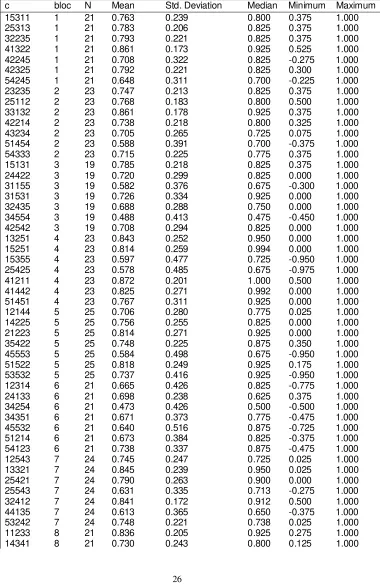
3.1.2 Health sta te values
In all there were 2455 health state valuations generated by the respondents. Average
number of valuations per intermediate health state was 22 (range from 19 to 22) where as
the ‘pits’ state (AQL-5D state 55555) was valued 307 times, by every respondent. The
mean health state values ranged from 0.39 to 0.94 and generally have fairly large standard
deviations (around 0.2 to 0.4). The distribution of the values was negatively skewed. Table
4 presents health valuation values in blocks 1 to 7 as examples (results of remaining states
3.2 Modelling
3.2.1 The main regression results
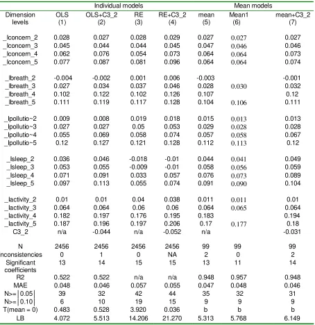
The results of modelling are presented in Table 5, with summary statistics for internal
sample predictions presented in the lower half of the table. Models (1) to (4) were estimated
at the individual level while models (5) to (7) were mean models estimated at the aggregate
level. Models were estimated on the basis of the main effects dummies except those with
the interaction variable C3_2. A fixed effects model was not present here as Hausman’s test
suggested random effects rather than fixed effects model.
For theoretical reasons, ‘the best model’ should be chosen between models that exclude the
constant term. Thus all models were estimated without constant terms. Among those
models estimated, individual level models (1) and (2) have no inconsistencies within
significant coefficients, whereas mean model (5) has 2. The number of significant
coefficients among models is comparable (range from 13 to 15). Given different
observation basis, the adjusted R2 values between individual models and mean models are
not comparable with each other. In terms of prediction ability, model (1) and model (5)
performed equally well with comparable MAE (0.048 vs. 0.047), numbers of absolute
residuals larger than 0.05 (39 vs. 35) and 0.10 (6 vs. 9), while model (3) performed worse
than them with larger MAE (0.057), more residuals larger than 0.05 (42) and 0.10 (19).
Ljung-Box test has been used to test autocorrelation between errors. The results showed
Introduction of interaction term C3_2 in the main effects models resulted in models (2), (4)
and (7). The coefficients for C3_2 term were non-significant for models (2) and (7), while
significant for model (4) with a negative sign. However, inclusion of C3_2 did not result in
appreciable change to the size of the main effects coefficients, nor any improvement of
prediction ability. In fact, the residual T-test for models (2) and (3), and the LB test for
model (4) became significant while main effects model were non-significant. Thus, the
interaction term C3_2 was not to be included in the final model.
Given the main purpose of modelling is to predict mean TTO values of all possible health
states defined by AQL-5D based on the valuation survey, the predictive ability of models
was used as the main criteria for model comparison and selection. As a result, the choice of
model is between model (1) (OLS model) and model (5) (Mean model), which have equally
good predictive ability. The mean model (5) is chosen as the best model, because health
state values required in economic evaluation are the average values of specific health states,
which means the aggregate level rather than the individual level. However, model (5) has 3
inconsistent coefficients - between breath level 1 as baseline and level 2, between breath
levels 4 and 5, and between activity levels 4 and 5, so these inconsistent levels were merged
to improve coefficient consistency, which resulted in model (6). Model (6) is the final
recommended model for use in future economic evaluations.
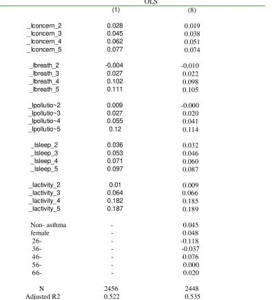
3.2.2 The additional analyses
Table 6 presents the OLS models before (model (1)) and after (model (8)) covariates
adjusted R square did not change remarkably after including covariates (0.522 vs. 0.535).
Most main effects coefficients showed very minor change at 0.001 level while the
coefficients within sleep dimension seemed to be most affected.
In model (8), the coefficient for not having asthma is 0.045 (p < 0.05). This indicates that
asthma patients have lower dis_TTO values than the general public, which means they are
on average giving higher values to asthma states. The coefficient for gender is 0.048
(p<0.05). This indicates that females have higher dis_TTO values than males, which means
they are on average giving lower values to health states. These two coefficients were
similar in size which may indicates that asthma condition and gender have similar effects
on the model. Further, the coefficients for age groups ranged from -0.118 to 0.020, with
groups 26 to 35 and 46 to 55 had negative values and were significant at 0.05 level, which
indicates that those two age groups in general gave higher values to health states. The
coefficients of other age groups were non-significant at 0.05 level.
4. Discussion and conclusion
This paper presents a study to estimate a preference-based single index from a condition
specific quality of life instrument, using the AQLQ. This means that it is possible to
convert AQLQ data sets into health state utility values for use in economic evaluations.
The alleged advantage of condition specific preference-based measures over generic ones is
that they use a descriptive system that is more relevant and sensitive to the condition.
condition specific measures for use in making cross programme comparison (Brazier et al,
2007)
A related issue is the choice of condition specific full health (AQL-5D state 11111) as
opposed to generic “full health” as the upper anchor for TTO valuation. Given that it is
quite possible to conceive of health states that involve no respiratory problems (and hence
correspond to AQL-5D 11111), and yet involve other health problems (e.g. pain), an
alternative design would be to use a generic description such as “no health problems” as the
upper TTO anchor and to directly evaluate AQL-5D 11111 against this and death. The
difficulty with this is that since the other dimensions of health are not explicitly mentioned,
it could be confusing to respondents.
We do not know what respondents were thinking during the interview: did they only think
about the condition as described by AQL-5D, or did they extend their imagination to other
aspects of health not included by in the descriptive system, such as depression or pain.
Respondents might imagine that other dimensions are either at their best level, or some
level constant between AQL-5D states (such as their current health), then provided there
are no interactions between those states that are included in the AQL-5D and those
dimensions excluded from its descriptive system, then this should not matter. However,
there is a good chance that there are interactions between these dimensions, and without
further data we can not know how important these are likely to be. In addition, if the levels
given to these other dimensions of health were related to the main asthma specific
pain and very depressed for the severe asthma states), then this would also have
implications for the final health state values
On more specific design issues, the selection of the health state sample for valuation and
modelling was based on balanced design regardless of the prevalence of health state in
population, which may cause difficulty for respondents to imagine those health states
happened rarely in real life. We checked the feasibility of the states and none seemed to
cause any problems for respondents. Further, the sample size of over 300 might be thought
to be small compared the original EQ-5D valuation survey with a sample of 3000, given the
AQL-5D descriptive system defines 13 times more health states than the EQ-5D. We were
limited by resource constraints since the collection of stated preference data by interview is
expensive. However, in terms of MAE, the results are both around 0.05 and the chosen
model did not suffer from many inconsistencies. A larger sample size with more states
may have allowed us to estimate significant interaction terms, but the additive model
seemed to perform satisfactorily against conventional statistical tests
The additional regression analyses introduce covariance of gender, age and asthma
condition into the OLS model. Although the coefficients of the main effects variables
mainly remain unchanged, the gender variable is statistically significant. Two age groups
are also significantly different from the reference age group (18 to 25), which indicates that
older people of specific age group were giving higher values. Nevertheless, these results
The impact of patients’ asthma condition to health state valuation has also been examined
by using a variable to represent whether or not the respondent has asthma in the OLS
models. This resulted in the coefficients being significant and being positive in the model.
This indicates that there was statistically significant difference between the way
respondents with and without asthma valued the hypothetical asthma states. Further,
respondents with asthma valued the hypothetical asthma states higher than those without
asthma, which has been confirmed by findings elsewhere (e.g. Dolan and Roberts, 2004).
The possible explanation may be that asthma patients have adapted the condition although
they know better of the condition than non-patients. These findings are similar to paper on
EQ-5D and SF-6D found gender, age and health status did have significant impact though
usually quite modest compared to the descriptive system. (Dolan and Roberts, Kharoubi et
al, 2007)
Given people with asthma gave different values; this does raise of the question of the extent
to which the general public understood the impact of the condition as discussed below.
Since the preference indices for a specific medical condition was valued by members of the
general public, one concern is the extent to which the majority of respondents who have no
direct experience of asthma managed to understand and to imagine what it is like to live
with asthma.
For informing resource allocation purposes, most agencies require values from a
representative population and so this is not relevant. However, we did undertake a pilot
had no effect. However, this study found that asthma condition does have an impact on the
final results.
In conclusion, this paper is one of the first to present the results from a study to derive a
condition-specific preference-based measure from an existing measure of health related
quality of life. While the study has been a technical success, it does raise some important
policy issues about the use of preference-based condition specific measures compared to
References
Anderson JP, Kaplan RM, Berry CC, et al.Interday reliability of function assessment for a health-status measure - the Quality of Well-being Scale. Medical care 1989; 27 (11): 1076 -1084.
Brazier J, Roberts J, Deverill M. The estimation of a utility based algorithm from the SF-36 Health Survey. Journal of Health Economics 2002: 21:271- 292.
Brazier JE, Czoski-Murray C, Roberts J, Brown M, Symonds T, Kelleher C. Estimation of a preference-based index from a condition specific measure: the King's Health Questionnaire. Medical Decision Making (2007, in
press)
Brazier JE, Ratcliffe J, Tsuchiya A, Solomon J. Measuring and valuing health for economic evaluation. Oxford: Oxford University Press 2007.
Dolan P. Modelling valuation for Euroqol health states. Medical Care 1997;35:351-363.
Dolan P, Gudex C, Kind P. Valuing health states: A comparison of methods. Journal of Health Economics. 1996;2:209-232.
Dowie J. Decision validity should determine whether a generic or condition-specific HRQOL measure is used in health care decisions. Health Economics 2002; 11:1-8.
Eccles M, Grimshaw J, Steen N, Parkin D, Purves I, McColl E, et al. The design and analysis of a randomized controlled trial to evaluate computerized decision support in primary care: the COGENT study. Family Practice 2000;17(2):180-186
Gudex C. Time Trade-Off User Manual: Props and Self-Completion Methods. Centre for Health Economics, 1994
Juniper EF, Guyatt GH, Ferrie PJ, Griffith LE. Measuring quality of life in asthma. American Review of Respiratory Disease 1993; 147: 832 - 838.
Juniper EF, Buist AS, Cox FM, Ferrie PJ, King DR. Validation of a standardized version of the Asthma Quality of Life Questionnaire. Chest 1999;115(5):1265-1270.
Revicki DA, Leidy NK, et al. Development and preliminary validation of the multiattibute Rhinitis Symptom Utility Index. Quality of life research 1998; 7: 693-702.
Revicki DA, Leidy NK, et al. Intergrating patient preferences into health outcomes assessment: the
multiattribute Asthma Symptom Utility Index. Chest 1998; 114:998-1007.
Roberts J, Dolan P. To what extent do people prefer health states with higher values? A note on evidence from the EQ-5D valuation set. Health Economics 2004; 13(7):733-737.
Stolk EA, Busschbach JJV. Validity and feasibility of the use of condition-specific outcome measures in economic evaluation. Quality of life reseach 2003 (12): 363 – 371.
Torrance EA, Kereseci MA, et al. Development and initial validation of a new preference-based disease-spedific health related quality of life instrument form erectile function. Quality of life research 2004; 13:349-359.
Table 1: Standardized AQLQ items (taken from Juniper, 1993)
Item No. Question (during the last 2 weeks) as a result of your asthm a Domain Wording 1 Limited strenuous activities Activity Limitations 2 Limited moderate activities Activity Limitations 3 Limited social activities Activity Limitations 4 Limited work-related activities Activity Limitations 5 Limited sleeping Activity Limitations 6 How much discomfort or distress as a result of chest tightness Symptoms Quantity 7 Feel concerned about having asthma Emotional Time 8 Feel short of breath as a result of your asthma Sym ptoms Time 9 Experience asthma symptoms as a result of being exposed to cigarette
smoke
Environment Time 10 Experience a wheeze in your chest Symptoms Time 11 Feel you had to avoid a situation or environment because of cigarette
smoke
Activity Time 12 How much discomfort or distress have you felt as a result of coughing Symptoms Quantity 13 Feel frustrated as a result of your asthma Emotional Time 14 Experience a feeling of chest heaviness Symptoms Time 15 Feel concerned about the need to use medication for your asthma Emotional Time 16 Feel the need to clear your throat Symptoms Time 17 Experience asthma symptoms as a result of being exposed to dust Environment Time 18 Experience difficulty breathing out as a result of your asthm a Sym ptoms Time 19 Feel you had to avoid a situation or environment because of dust Activity Time 20 Wake up in the morning with asthma symptoms Symptoms Time 21 Feel afraid of not having your asthma medication available Emotional Time 22 Feel bothered by heavy breathing Sym ptoms Time 23 Experience asthma symptoms as a result of the weather or air pollution
outside
Environment Time 24 Were you woken at night by your asthma Symptoms Time 25 Avoid or limit going outside because of the weather or air pollution Activity Time 26 Experience asthma symptoms as a result of being exposed to strong
smells or perfume
Environment Time 27 Feel afraid of getting out of breath Emotional Time 28 Feel you had to avoid a situation of environment because of strong smells
or perfume
Activity Time 29 Has your asthma interfered with a good night’s sleep Symptoms Time 30 Have a feeling of fighting for air Sym ptoms Time 31 How much has your range of activities you would like to have done been
limited by your asthm a
Activity Limitations 32 Among all the activities you have done how limited have you been by your
asthma
Table 2 the reduced asthma quality of life classification (AQL-5D)
CONCERN
1. Feel concerned about having asthma none of the time.
2. Feel concerned about having asthma a little or hardly any of the time. 3. Feel concerned about having asthma some of the time.
4. Feel concerned about having asthma most of the time. 5. Feel concerned about having asthma all of the time.
SHORT OF BREATH
1. Feel short of breath as a result of asthma none of the time.
2. Feel short of breath as a result of asthma a little or hardly any of the time. 3. Feel short of breath as a result of asthma some of the time.
4. Feel short of breath as a result of asthma most of the time. 5. Feel short of breath as a result of asthma all of the time.
WEATHER & POLLUTION
1. Experience asthma symptoms as a result of air pollution none of the time.
2. Experience asthma symptoms as a result of air pollution a little or hardly any of the time. 3. Experience asthma symptoms as a result of air pollution some of the time.
4. Experience asthma symptoms as a result of air pollution most of the time. 5. Experience asthma symptoms as a result of air pollution all of the time.
SLEEP
1. Asthma interferes with getting a good night’s sleep none of the time.
2. Asthma interferes with getting a good night’s sleep a little or hardly any of the time. 3. Asthma interferes with getting a good night’s sleep some of the time.
4. Asthma interferes with getting a good night’s sleep most of the time. 5. Asthma interferes with getting a good night’s sleep all of the time.
ACTIVITIES
1. Overall, not at all limited with all the activities done. 2. Overall, a little limitation with all the activities done.
Table 3 Characteristics of respondents in evaluation survey (N=307)
Count Percentage
Age
18- 34 11.1
26- 57 18.6
36- 61 19.9
46- 50 16.3
56- 45 14.7
66- 60 19.5
Female 168 54.7
Have asthma 53 17.3
Married or living with partner 214 69.8
Experienced serious illness:
in family 194 63.4
themselves 94 30.6
Degree or equivalent 69 22.5
Education after 17 140 45.6
Renting property 64 20.8
Found valuation task difficult:
very difficult 24 7.9
quite difficult 82 26.7
Neither difficult nor easy 52 16.9
Self-reported EQ-5D score male female
Respondent sample 0.83 0.84
Table 4 Descriptive statistics for AQL-5D health state values (blocks 1 to 14)
c bloc N Mean Std. Deviation Median Minimum Maximum
15311 1 21 0.763 0.239 0.800 0.375 1.000
25313 1 21 0.783 0.206 0.825 0.375 1.000
32235 1 21 0.793 0.221 0.825 0.375 1.000
41322 1 21 0.861 0.173 0.925 0.525 1.000
42245 1 21 0.708 0.322 0.825 -0.275 1.000
42325 1 21 0.792 0.221 0.825 0.300 1.000
54245 1 21 0.648 0.311 0.700 -0.225 1.000
23235 2 23 0.747 0.213 0.825 0.375 1.000
25112 2 23 0.768 0.183 0.800 0.500 1.000
33132 2 23 0.861 0.178 0.925 0.375 1.000
42214 2 23 0.738 0.218 0.800 0.325 1.000
43234 2 23 0.705 0.265 0.725 0.075 1.000
51454 2 23 0.588 0.391 0.700 -0.375 1.000
54333 2 23 0.715 0.225 0.775 0.375 1.000
15131 3 19 0.785 0.218 0.825 0.375 1.000
24422 3 19 0.720 0.299 0.825 0.000 1.000
31155 3 19 0.582 0.376 0.675 -0.300 1.000
31531 3 19 0.726 0.334 0.925 0.000 1.000
32435 3 19 0.688 0.288 0.750 0.000 1.000
34554 3 19 0.488 0.413 0.475 -0.450 1.000
42542 3 19 0.708 0.294 0.825 0.000 1.000
13251 4 23 0.843 0.252 0.950 0.000 1.000
15251 4 23 0.814 0.259 0.994 0.000 1.000
15355 4 23 0.597 0.477 0.725 -0.950 1.000
25425 4 23 0.578 0.485 0.675 -0.975 1.000
41211 4 23 0.872 0.201 1.000 0.500 1.000
41442 4 23 0.825 0.271 0.992 0.000 1.000
51451 4 23 0.767 0.311 0.925 0.000 1.000
12144 5 25 0.706 0.280 0.775 0.025 1.000
14225 5 25 0.756 0.255 0.825 0.000 1.000
21223 5 25 0.814 0.271 0.925 0.000 1.000
35422 5 25 0.748 0.225 0.875 0.350 1.000
45553 5 25 0.584 0.498 0.675 -0.950 1.000
51522 5 25 0.818 0.249 0.925 0.175 1.000
53532 5 25 0.737 0.416 0.925 -0.950 1.000
12314 6 21 0.665 0.426 0.825 -0.775 1.000
24133 6 21 0.698 0.238 0.625 0.375 1.000
34254 6 21 0.473 0.426 0.500 -0.500 1.000
34351 6 21 0.671 0.373 0.775 -0.475 1.000
45532 6 21 0.640 0.516 0.875 -0.725 1.000
51214 6 21 0.673 0.384 0.825 -0.375 1.000
54123 6 21 0.738 0.337 0.875 -0.475 1.000
12543 7 24 0.745 0.247 0.725 0.025 1.000
13321 7 24 0.845 0.239 0.950 0.025 1.000
25421 7 24 0.790 0.263 0.900 0.000 1.000
25543 7 24 0.631 0.335 0.713 -0.275 1.000
32412 7 24 0.841 0.172 0.912 0.500 1.000
44135 7 24 0.613 0.365 0.650 -0.375 1.000
53242 7 24 0.748 0.221 0.738 0.025 1.000
11233 8 21 0.836 0.205 0.925 0.275 1.000
14444 8 21 0.529 0.451 0.575 -0.875 1.000
23154 8 21 0.714 0.276 0.800 0.000 1.000
33323 8 21 0.818 0.227 0.900 0.275 1.000
42554 8 21 0.571 0.457 0.725 -0.825 1.000
54152 8 21 0.701 0.382 0.875 -0.500 1.000
21332 9 19 0.850 0.221 0.925 0.400 1.000
22242 9 19 0.801 0.237 0.900 0.225 1.000
24433 9 19 0.715 0.305 0.825 0.025 1.000
32441 9 19 0.833 0.256 0.925 0.075 1.000
44114 9 19 0.562 0.513 0.725 -0.950 1.000
45143 9 19 0.704 0.301 0.725 0.025 1.000
45253 9 19 0.663 0.446 0.725 -0.775 1.000
13431 10 25 0.798 0.228 0.900 0.200 1.000
21113 10 25 0.885 0.133 0.925 0.450 1.000
23534 10 25 0.633 0.286 0.625 0.000 1.000
41125 10 25 0.685 0.248 0.725 0.000 1.000
41153 10 25 0.733 0.308 0.800 -0.400 1.000
53325 10 25 0.540 0.381 0.575 -0.300 1.000
53525 10 25 0.467 0.419 0.500 -0.700 1.000
13514 11 23 0.691 0.265 0.700 0.125 1.000
24335 11 23 0.629 0.278 0.650 0.000 1.000
31143 11 23 0.805 0.201 0.875 0.325 1.000
41112 11 23 0.891 0.164 0.950 0.425 1.000
45341 11 23 0.769 0.273 0.875 0.075 1.000
52444 11 23 0.699 0.214 0.700 0.300 1.000
53411 11 23 0.827 0.192 0.925 0.375 1.000
23312 12 21 0.937 0.105 1.000 0.600 1.000
24352 12 21 0.875 0.175 0.925 0.325 1.000
33511 12 21 0.900 0.135 1.000 0.500 1.000
33552 12 21 0.849 0.194 0.925 0.300 1.000
52112 12 21 0.934 0.127 1.000 0.525 1.000
52314 12 21 0.855 0.201 0.925 0.325 1.000
55424 12 21 0.780 0.220 0.825 0.375 1.000
13434 13 20 0.586 0.407 0.700 -0.575 1.000
15331 13 20 0.830 0.166 0.825 0.525 1.000
24524 13 20 0.486 0.500 0.563 -0.575 1.000
35453 13 20 0.614 0.387 0.625 -0.375 1.000
41123 13 20 0.805 0.313 0.912 -0.425 1.000
52141 13 20 0.840 0.314 0.963 -0.375 1.000
55521 13 20 0.578 0.459 0.688 -0.475 1.000
11445 14 22 0.696 0.235 0.713 0.225 1.000
12511 14 22 0.819 0.228 0.938 0.375 1.000
15553 14 22 0.701 0.376 0.800 -0.475 1.000
31215 14 22 0.712 0.257 0.763 0.225 1.000
32414 14 22 0.672 0.357 0.787 -0.400 1.000
33245 14 22 0.717 0.264 0.750 0.225 1.000
34225 14 22 0.641 0.367 0.675 -0.475 1.000
Table 5 Main models Estimated
Individual models Mean models
Dimension levels OLS (1) OLS+C3_2 (2) RE (3) RE+C3_2 (4) mean (5) Mean1 (6) mean+C3_2 (7)
_Iconcern_2 0.028 0.027 0.028 0.029 0.027 0.027 0.027 _Iconcern_3 0.045 0.044 0.044 0.045 0.047 0.046 0.046 _Iconcern_4 0.062 0.076 0.054 0.073 0.064 0.064 0.073 _Iconcern_5 0.077 0.087 0.081 0.096 0.064 0.064 0.074
_Ibreath_2 -0.004 -0.002 0.001 0.006 -0.003 -0.001
_Ibreath_3 0.027 0.034 0.037 0.046 0.028 0.030 0.032
_Ibreath_4 0.102 0.122 0.102 0.126 0.107 0.12
_Ibreath_5 0.111 0.119 0.117 0.128 0.104 0.106 0.111
_Ipollutio~2 0.009 0.008 0.019 0.018 0.015 0.013 0.013 _Ipollutio~3 0.027 0.027 0.05 0.053 0.029 0.028 0.028 _Ipollutio~4 0.055 0.069 0.058 0.074 0.057 0.058 0.067 _Ipollutio~5 0.12 0.127 0.121 0.128 0.112 0.113 0.12
_Isleep_2 0.036 0.046 -0.018 -0.01 0.044 0.041 0.049 _Isleep_3 0.053 0.055 -0.009 -0.01 0.058 0.056 0.059
_Isleep_4 0.071 0.091 0.033 0.057 0.076 0.073 0.089
_Isleep_5 0.097 0.113 0.055 0.074 0.091 0.090 0.104
_Iactivity_2 0.01 0.01 0.04 0.038 0.011 0.011 0.01
_Iactivity_3 0.064 0.064 0.06 0.06 0.064 0.065 0.064
_Iactivity_4 0.182 0.197 0.176 0.195 0.183 0.194
_Iactivity_5 0.187 0.196 0.197 0.206 0.17 0.177 0.18
C3_2 n/a -0.044 n/a -0.052 n/a -0.031
N 2456 2456 2456 2456 99 99 99
Inconsistencies 0 1 0 NA 2 0 2
Significant coefficients
13 14 15 15 13 11 14
R2 0.522 0.522 n/a n/a 0.948 0.957 0.948
MAE 0.048 0.046 0.057 0.055 0.047 0.048 0.046
N>= 0.05 39 32 42 44 35 32 31
N>= 0.10 6 10 19 15 9 9 9
T(mean = 0) 0.483 0.528 3.920 0.036 b b b
LB 4.072 5.513 14.206 21.270 5.313 5.768 6.149
Note:
All models used dis_tto as dependent variable. All models were estimated without constant Estimates shown in bold are significant at P0.05
C3-2 is an interaction term with 1 denoting two or more dimensions in a health states greater than level 4, 0 otherwise.
Table 6 OLS model with covariates
OLS
(1) (8)
_Iconcern_2 0.028 0.019
_Iconcern_3 0.045 0.038
_Iconcern_4 0.062 0.051
_Iconcern_5 0.077 0.074
_Ibreath_2 -0.004 -0.010
_Ibreath_3 0.027 0.022
_Ibreath_4 0.102 0.098
_Ibreath_5 0.111 0.105
_Ipollutio~2 0.009 -0.000
_Ipollutio~3 0.027 0.020
_Ipollutio~4 0.055 0.041
_Ipollutio~5 0.12 0.114
_Isleep_2 0.036 0.032
_Isleep_3 0.053 0.046
_Isleep_4 0.071 0.060
_Isleep_5 0.097 0.087
_Iactivity_2 0.01 0.009
_Iactivity_3 0.064 0.066
_Iactivity_4 0.182 0.185
_Iactivity_5 0.187 0.189
Non- asthma - 0.045 female - 0.048
26- - -0.118 36- - -0.037 46- - -0.076
56- - 0.000
66- - 0.020
N 2456 2448 Adjusted R2 0.522 0.535
All models used dis_tto as dependent variable. All models were estimated without constant Estimates shown in bold are significant at P0.05
Appendix 1: the infor mation on asthma shown to r espondents
What is asthma?
Asthma is a condition that affects the airways - the small tubes that carry air in and out of the lungs. If you have asthma your airways are almost always sensitive and inflamed.
When you come in to contact with something you are allergic to, or something that irritates your airways (a trigger), you airways will become narrower, making it harder to breathe. The muscles around the walls of your airways tighten. The lining of the airways becomes inflamed and starts to swell and often sticky mucus or phlegm is produced. This will lead to you experiencing asthma symptoms.
Asthma symptoms can vary. You may find that you start to cough or wheeze, get short of breath, or have a tight feeling in your chest. Despite what many people think, wheezing does not always occur. In fact, coughing is the most common asthma symptom.
Asthma can start at any age. Some people get symptoms during childhood which then disappear in later life. Others develop ‘late-onset’ asthma in adulthood, without ever having had symptoms as a child.
Appendix 2:
Estimating a single utility index from the Mini Asthma Quality of Life Questionnaire (MiniAQLQ) using the AQL-5D
The MiniAQLQ has been developed and fully validated by Professor Juniper and her
colleagues, who has also developed the Asthma Quality Life Questionnaire (AQLQ), in
response to a demand for a shorter, standardized version for large clinical trials and for
managed care monitoring (Juniper et al, 1999). This instrument has 15 items and each
item has the same 7 severity levels as the original AQLQ. The items are in the same
domains as the original AQLQ (5 items for the symptoms domain, 4 items for the
activities domain, 3 items for the emotions domain and 3 items for the environment
domain). Most items are identical to the corresponding items of the original AQLQ
although some items have slightly different wording. The MiniAQLQ has very good
reliability, cross-sectional validity, responsiveness and longitudinal validity (Juniper et al,
1999).
Although the AQL-5D was derived from the AQLQ, given the large overlap between the
AQLQ and the MiniAQLQ questionnaires, the AQL-5D can also be used to derive utility
indices from MiniAQLQ data. Four of the 5 AQL-5D dimensions (concern, short of
breath, weather & pollution dimensions) have identical MiniAQLQ items. In terms of the
activity limitation dimension, the AQL-5D question (item 32 of AQLQ) asks about
limitations in all activities that the respondent has undertaken in the last 2 weeks. While
there are 4 items relating to activity limitation in the MiniAQLQ, none of them ask the
same question. They ask how asthma limited respondents in the last 2 weeks doing
different activities: strenuous activities (item 12), moderate activities (item 13), social
activities (item 14) and work-related activities (item 15).
In this appendix, 4 different approaches for specifying a level of the AQL-5D activity
dimension based on the MiniAQLQ activities items are compared.
1. Average of items 13-15 rounded up;
3. Take item 13 as is;
4. Take the worst item from items 13 -15.
Averages are rounded up in approaches 1 and 2 because the AQL-5D algorithm is only
applicable to round numbers.
Since item 12 (limited strenuous activity) may not represent the level of a respondent’s
overall activity limitation, this item was only considered in approach 2. Among these 4
approaches, approach 1 took moderate, social and work-related activity limitation into
account and we believe is the most appropriate way to obtain the activity dimension of
AQL-5D from the MiniAQLQ. Three other approaches were developed to test the
sensitivity of the utility values to different assumptions.
The 4 approaches have been applied to the baseline data of a trial containing MiniAQLQ
(Lloyd et al, 2007). Table 1 reports AQL-5D health state values resulting from the 4
approaches. The results show little difference between values which range from 0.787
(approach 4) to 0.802 (approach 1). In terms of distribution of values, the median and 20
percentiles resulting from these 4 approaches are also very close to each other.
Table 1 Description for health state values resulting from 4 approaches
Approach 1 Approach 2 Approach 3 Approach 4
N 106 106 106 106
Mean 0.802 0.794 0.798 0.787
Median 0.826 0.822 0.822 0.807 Std. Deviation 0.131 0.134 0.130 0.131 Minimum 0.450 0.450 0.450 0.450 Maximum 0.970 0.970 0.970 0.970 20 0.714 0.698 0.698 0.690 40 0.794 0.790 0.790 0.777 60 0.863 0.849 0.859 0.836 Percentiles
80 0.922 0.917 0.921 0.913
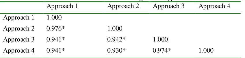
Pearson correlation coefficients were calculated for utility values resulting from these 4
significant at the 0.01 level. The Intra Class Correlation (ICC) analysis across these
[image:37.595.83.507.170.272.2]approaches results in a coefficient as 0.949 and is significant at 0.01 significant level.
Table 2 Correlation coefficients for values resulting from 4 approaches
Approach 1 Approach 2 Approach 3 Approach 4
Approach 1 1.000
Approach 2 0.976* 1.000
Approach 3 0.941* 0.942* 1.000
Approach 4 0.941* 0.930* 0.974* 1.000
* Correlation is significant at 0.01 level (2 tailed)
The above analysis shows that results from approach 1 and the other approaches were of
little difference in terms of mean and median values, as well as distribution of indices. In
fact, the results were closely correlated as shown by Pearson and ICC correlation
coefficients. Thus, the approach 1 is recommended as a practical solution.
A SPSS syntax file to calculate utility indices from the MiniAQLQ questionnaire based
on approach 1 is available from the authors on request.
Reference:
1.
JJuniper EF, Guyatt GH, Cox FM, Ferrie PJ, King DR. Development and validation of the Mini Asthma Quality of Life Questionnaire. European Respiratory Journal1999; 14: 32-38