A Method to Simulate the Skew Normal Distribution

(1)

http://dx.doi.org/10.4236/am.2014.513201

A Method to Simulate the Skew Normal

Distribution

Dariush Ghorbanzadeh, Luan Jaupi, Philippe Durand CANAM-Département IMATH, Paris, France

Email: [email protected], [email protected], [email protected]

Received 2 May 2014; revised 10 June 2014; accepted 17 June 2014

This work is licensed under the Creative Commons Attribution International License (CC BY). http://creativecommons.org/licenses/by/4.0/

Abstract

A new method is developed to simulate the skew normal distribution. The result is interesting from a practical as well as a theoretical viewpoint. The new method is simple to program and is more efficient than the standard method of simulation by acceptance-rejection method.

Keywords

Normal Distribution, Skew Normal Distribution

1. Introduction

In this paper, we denote by SN

( )

θ the skew normal distribution of parameter θ and density :

( )

2

( ) ( )

f x = ϕ x Φ θx (1) where ϕ and Φ denote the standard normal 

( )

0,1 probability density function and cumulative distribu-tion funcdistribu-tion, respectively.

The skew normal distribution, due to its mathematical tractability and inclusion of the standard normal distri-bution, has attracted a lot of attention in the literature. Azzalini [1], Azzalini [2], Chiogna [3], Genton & Liu [4] and Henze [5] discussed basic mathematical and probabilistic properties of the skew normal family. The multi-variate skew normal distribution is studied by Azzalini & Capitanio [6] and Azzalini & Dalla Valle [7]. For ad-ditional references and a review on related literature, see Azzalini & Capitanio [8] and Pewsey [9] for a collec-tion of papers on the subject. Henze [5], in his paper showed that if U1 and U2 are identically and indepen- dently distributed 

( )

0,1 random variables, then 1 2

2

1

U U

θ θ +

+ has the skew normal distribution.

(2)

D. Ghorbanzadeh et al.

2074

the independent and identically distributed 

( )

0,1 random variables.

2. Method

Let U1 and U2 two independent and identically distributed 

( )

0,1 random variables and U=max

(

U U1, 2

)

and V =min

(

U U1, 2

)

. For simulation of the random variable XSN

( )

θ , we take the combination of U and

V. First note that:

• if θ=0, the density (1) becomes: f x

( )

=ϕ

( )

x , simply simulate X

( )

0,1 . • if θ = −1, the density (1) becomes: f x

( )

=2ϕ

( )

x

(

1− Φ

( )

x

)

, we take X =V . • if θ =1, the density (1) becomes: f x

( )

=2ϕ

( ) ( )

x Φ x , we take X =U.

For θ∈ −/

{

1, 0,1

}

, note :

(

)

(

)

1 2

2 2

1 1

,

2 1 2 1

θ θ

λ λ

θ θ

+ −

= =

+ + (2)

We note that: λ12+λ22=1. For simulation of the random variable X SN

( )

θ , we take the combination of

U and V in the form:

1 2

X =λU+λV (3)

Proposition The random variable X defined in the Equation (3) has the skew normal distribution SN

( )

θ . Proof. The pair

(

U V,

)

has density: f_{U V}_,

( )

u v, =2ϕ

( ) ( )

u ϕ v ll_{_{v u}_≤_}

( )

u v, , where ll is the indicator function. Consider the transformation: x=λ1u+λ2v y, =λ1u. The inverse transform is defined by:

1 2

,

y x y

u v

λ λ

−

= =

and the corresponding Jacobian is:

1 2 1 J

λ λ

= . X density is defined by:

( )

1 2 1 2

2

d

y x y f x ϕ ϕ y

λ λ ∆ λ λ

   − 

= _{  } _

   

∫

(4)

where

2 1

x y y

λ λ

 − 

∆ = ≤ 

 . Taking into account

2 2

1 2 1

λ +λ = , we can write:

( )

12

1 2 1 2

y x y x y

x λ

ϕ ϕ ϕ ϕ

λ λ λ λ

 

   − ₌ −

 

    _ _

      (5)

Equation (4) becomes,

( )

12

1 2 1 2

2

d

x y x f x ϕ ϕ λ y

λ λ ∆ λ λ

 − 

= _ _

 

∫

(6)

For the domain ∆, we have the following three cases:

Case 1: θ∈ −

(

1, 0

) ( )

 0,1 , we have:

(

)

2

1 2 2

1 2 1 θ λ λ θ − =

+ and

1 1 2 x y λ λ λ   ∆ = ≥ ₊   

Case 2: θ< −1, we have:

) 2(1 1 = | | ₂ 2 2 1 _θ θ λ λ + −

and 1

1 2 x y λ λ λ   ∆ =_ ≥ _ +  

Case 3: θ>1, we have:

) 2(1 1 = | | ₂ 2 2 1 _θ θ λ λ + −

and 1

1 2 x y λ λ λ   ∆ =_ ≤ _ +  

Using Equation (6) and the three cases above, we get the result.

3. Simulation Results

(3)

andTable 1,Table 2 show the results obtained by our method and the method Henze [5].

The results of Table 1 andTable 2 show that our method provides results close to the theoretical values and secondly, we obtain results similar to those obtained by Henze [5] results.

4. Conclusion

[image:3.595.89.538.183.311.2]

In this article we propose a very simple method to simulate skew normal family distribution. The obtained

Table 1. Simulation results for a sample size of 500,000 and θ = −7.

θ = −7

Theoretical value Simulated valuea _{Simulated value}b

Mean −0.789865 −0.789651 −0.790496

Variance 0.376113 0.375669 0.376671

Skewness −0.916950 −0.915649 −0.924019

Kurtosis 0.779197 0.768095 0.796781

[image:3.595.89.539.350.471.2]

a_{by our method;}b_{by the method of Henze}_[5]_.

Table 2. Simulation results for a sample size of 500,000 and θ = 13.

θ = 13

Theoretical value Simulated valuea _{Simulated value}b

Mean 0.795534 0.795174 0.795930

Variance 0.367125 0.366461 0.367464

Skewness 0.971447 0.969756 0.970813

Kurtosis 0.841547 0.836937 0.831219

a

by our method; bby the method of Henze [5].

(a) (b)

[image:3.595.87.540.409.687.2]

(4)

D. Ghorbanzadeh et al.

2076

[image:4.595.98.538.81.276.2]

(a) (b)

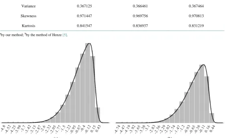
Figure 2. Histogram of simulations for a sample size of 500,000 and θ = 13. (a) histogram of simulations using our method; (b) histogram of simulations using the method of Henze [5].

results are very close to theoretical values and the method is more efficient than the standard one. The method is simple to program and exploit for practical applications.

References

[1] Azzalini, A. (1985) A Class of Distributions Which Includes the Normal Ones. Scandinavian Journal of Statistics, 12, 171-178.

[2] Azzalini, A. (1986) Further Results on the Class of Distributions Which Includes the Normal Ones. Statistica, 46, 199- 208.

[3] Chiogna, M. (1998) Some Results on the Scalar Skew-Normal Distribution. Journal of the Italian Statistical Society, 1, 1-13.http://dx.doi.org/10.1007/BF03178918

[4] Genton, M.G., He, L. and Liu, X. (2001) Moments of Skew Normal Random Vectors and Their Quadratic Forms. Sta-tistics & Probability Letters, 51, 319-325.http://dx.doi.org/10.1016/S0167-7152(00)00164-4

[5] Henze, N. (1986) A Probabilistic Representation of the Skew-Normal Distribution. Scandinavian Journal of Statistics,

13, 271-275.

[6] Azzalini, A. and Capitanio, A. (1999) Statistical Applications of the Multivariate Skew-Normal Distributions. Journal of the Royal Statistical Society, Series B, 61, 579-602.http://dx.doi.org/10.1111/1467-9868.00194

[7] Azzalini, A. and Dalla Valle, A. (1996) The Multivariate Skew-Normal Distribution. Biometrika, 83, 715-726.

http://dx.doi.org/10.1093/biomet/83.4.715

[8] Azzalini, A. and Capitanio, A. (2003) Distributions Generated by Perturbation of Symmetry with Emphasis on a Mul-tivariate Skew t Distribution. Journal of the Royal Statistical Society, Series B, 65, 367-389.

http://dx.doi.org/10.1111/1467-9868.00391

(5)

currently publishing more than 200 open access, online, peer-reviewed journals covering a wide range of academic disciplines. SCIRP serves the worldwide academic communities and contributes to the progress and application of science with its publication.