Hydrol. Earth Syst. Sci., 22, 4565–4581, 2018 https://doi.org/10.5194/hess-22-4565-2018 © Author(s) 2018. This work is distributed under the Creative Commons Attribution 4.0 License.
Incremental model breakdown to assess the multi-hypotheses
problem
Florian U. Jehn1, Lutz Breuer1,2, Tobias Houska1, Konrad Bestian1, and Philipp Kraft1
1Institute for Landscape Ecology and Resources Management (ILR), Research Centre for BioSystems, Land Use and Nutrition (iFZ), Justus Liebig University Giessen, Heinrich-Buff-Ring 26, 35390 Giessen, Germany
2Centre for International Development and Environmental Research (ZEU), Justus Liebig University Giessen, Senckenbergstraße 3, 35392 Giessen, Germany
Correspondence:Florian U. Jehn ([email protected]) Received: 27 November 2017 – Discussion started: 29 November 2017
Revised: 13 August 2018 – Accepted: 14 August 2018 – Published: 29 August 2018
Abstract. The ambiguous representation of hydrological processes has led to the formulation of the multiple hypothe-ses approach in hydrological modeling, which requires new ways of model construction. However, most recent studies focus only on the comparison of predefined model structures or building a model step by step. This study tackles the prob-lem the other way around: we start with one complex model structure, which includes all processes deemed to be impor-tant for the catchment. Next, we create 13 additional simpli-fied models, where some of the processes from the starting structure are disabled. The performance of those models is evaluated using three objective functions (logarithmic Nash– Sutcliffe; percentage bias, PBIAS; and the ratio between the root mean square error and the standard deviation of the mea-sured data). Through this incremental breakdown, we iden-tify the most important processes and detect the restraining ones. This procedure allows constructing a more streamlined, subsequent 15th model with improved model performance, less uncertainty and higher model efficiency. We benchmark the original Model 1 and the final Model 15 with HBV Light. The final model is not able to outperform HBV Light, but we find that the incremental model breakdown leads to a struc-ture with good model performance, fewer but more relevant processes and fewer model parameters.
1 Introduction
In the world of hydrological modeling, scientists construct models and apply them for a specific research question. Sometimes, these models are modified or extended after-wards, but the core components stay the same. This approach has existed from the earliest days of simple equations un-til the models of connected, conceptual elements used today (Todini, 2007).
During the development of hydrological models, the is-sues of parameter and input data uncertainty were often in the center of the scientific debate and numerous methods for assessing this uncertainty have been proposed. Structural un-certainty has been investigated in the past decade (Breuer et al., 2009; Son and Sivapalan, 2007) and gained more momen-tum in the last few years (e.g., Clark et al., 2015a; Fenicia et al., 2011; Hublart et al., 2015). It was noted that problems often arose from the focus on trying to build one model that was meant to work equally well for all catchments (Fenicia et al., 2011).
model should also be considered to better understand why a certain model works or fails (Clark et al., 2016).
When the idea of multiple hypotheses emerged, there was no easy way to construct models with interchangeable com-ponents (Buytaert et al., 2008), except for some comparison inside the TOPMODEL model family (Beven and Kirkby, 1979). However, Bergström (1991) already noted that a crit-ical view on the necessity of process descriptions is impor-tant in the development of models like HBV. We now have model frameworks at hand that facilitate such a design, e.g., SUPERFLEX (Fenicia et al., 2011), Structure for Unify-ing Multiple ModelUnify-ing Alternatives (SUMMA) (Clark et al., 2015a, b) or the Catchment Modelling Framework (CMF) (Kraft et al., 2011). SUPERFLEX targets the construction of lumped conceptual models (van Esse et al., 2013; Gharari et al., 2014). SUMMA and CMF support the generation of multi-scale approaches from plot over hillslope to basins and from lumped to fully distributed models. SUMMA fo-cusses on the comparison of process-based models with predefined parameter sets and is up to now mainly tested for surface–atmosphere interactions (Clark et al., 2015a, b). CMF is a programming library to build hydrological mod-els from building blocks with both process-based and con-ceptual models. It can be used for subsurface and surface water fluxes, surface–atmosphere exchange and solute trans-port. So far, it has been applied in studies to better understand hydrological processes (Holländer et al., 2009; Maier et al., 2017; Orlowski et al., 2016; Windhorst et al., 2014), to sim-ulate solute transport (Djabelkhir et al., 2017; Kraft et al., 2010), and to capture hydrological lateral and vertical trans-port processes in coupled complex ecosystem models (Haas et al., 2013; Houska et al., 2014, 2017; Kellner et al., 2017). All toolboxes enable a stepwise modification of the model structure. Additionally, they allow an easier comparison of different models, as they are all constructed from the same parts and are more straightforwardly handled through inter-faces (Buytaert et al., 2008). Recently, some studies tried to tackle the multi-hypotheses problem within a model frame-work (e.g., van Esse et al., 2013; Fenicia et al., 2008; Gharari et al., 2014; Hublart et al., 2015; Kavetski and Fenicia, 2011). Most of these studies built their models incrementally from the bottom up to find out if small modifications allow a better simulation (Bai et al., 2009; Westerberg and Birkel, 2015). Others compared predefined model structures (van Esse et al., 2013; Kavetski and Fenicia, 2011). In all cases, researchers stopped improving the models once a sufficient performance was reached. Clark et al. (2015a, b) propose an-other approach to test multiple hypotheses. Here, the num-ber and type of subprocesses stay static, yet the mathemati-cal formulation of the process descriptions are scrutinized by exchange. However, the different model-scrutinizing strate-gies are independent of the selected framework. SUMMA, SUPERFLEX, FUSE and CMF should be suitable for incre-mental model build-up, process exchange and our new pro-posal of the incremental model breakdown strategy.
Despite having the potential to create a wide range of models with such toolboxes, only a minor quantity in the vast space of possible model structures is currently explored. However, this thorough exploration is needed to find appro-priate model structures for any catchment, as it seems that current hydrological knowledge does not allow us to con-struct a model that works equally well for all environmen-tal conditions, especially when using lumped models (Beven, 2000, 2007, 2016; Buytaert et al., 2008; Fenicia et al., 2014). To better use the existing understanding of a given catch-ment and to test more complex models, this study turns the incremental approach of adding more process understand-ing to a model upside down. First, we develop a concep-tual model from current hydrological understanding that con-tains all subprocesses that might be important for the func-tioning of a catchment. Then, parts of this model are dis-abled through incremental model breakdown, and the re-duced model structures are tested for their simulation perfor-mance. A subprocess is marked as necessary when models lacking it are rejected. On this base, a subsequent model is constructed which uses only meaningful subprocesses. Incre-mental model breakdown is therefore a rejectionist approach, built on the learning from failure and not an optimization pro-cess. Beven (2006) assumed that a rejectionist approach is generally better suited to gain insight about process hypothe-ses. To allow comparability of the incremental breakdown method with common modeling approaches, the subsequent model is finally benchmarked with HBV Light.
The objective of this study is to demonstrate that incre-mental model breakdown allows a detailed examination of model structures, an easier identification of the most impor-tant hydrological processes and thus the construction of an improved model. While still not being able to sample the en-tire space of possible model structures, this approach might find some model structures which are likely missed with other methods. Ultimately, this approach also enables a bet-ter hydrological understanding of the catchment, as different structures, flaws and errors of a first modeling approach be-come obvious, even if a theoretical optimal model structure is still unknown.
2 Material and methods 2.1 Study area
F. U. Jehn et al.: Incremental model breakdown to assess the multi-hypotheses problem 4567
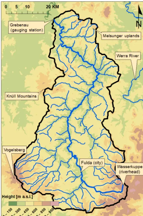
Figure 1.Relief map of the partial catchment of the Fulda River (black border) with side streams, ridges and parts of the Werra River.
for drinking water supply, sewage treatment works, reser-voirs or sealed areas).
Precipitation input is influenced by the surrounding low mountain ridges of the Vogelsberg, the Wasserkuppe, the Knüll Mountains and the Melsunger uplands, leading to a significant contribution of snowfall in winter. The elevation ranges from about 150 m a.s.l. at Grebenau to 950 m a.s.l. at the Wasserkuppe. Wittmann (2002) used tritium as a tracer and found that the Fulda catchment has two distinct ground-water reservoirs: a large one reacting slowly and a smaller one with faster reaction. Land use is dominated by agricul-ture (37 %) and forests (41 %).
2.2 Model input and validation data
Discharge data for the gauging station Grebenau, temper-ature and precipitation data were obtained from the Hes-sisches Landesamt für Naturschutz, Umwelt und Geologie (HLNUG). The point measurements for precipitation and temperature of the 51 measurement stations were
extrapo-Figure 2.Cumulative discharge plotted against cumulative precip-itation for the calibration (1980–1985) and validation (1986–1988) period and 2 years which deviate most from the other years. For the calibration and validation period, the cumulative discharge and precipitation are the average of the corresponding years.
lated over the whole catchment, using kriging with altitude as an external drift (Hudson and Wackernagel, 1994). Finally, the extrapolated values were averaged over the whole catch-ment to get a single, lumped value per day. The time period from 1979 to 1988 was chosen because external drift krig-ing requires a high density of precipitation stations and this mentioned period covered most measuring stations with con-tinuous data.
The Fulda catchment has a humid, temperate climate, with an annual precipitation of 838 mm. The annual runoff coef-ficient ranges between 0.3 and 0.6 (average 0.39), which is in the range for comparable catchments (e.g., Rawlins et al., 2006). The discharge and groundwater of the catchment are influenced by drinking water abstraction for 80 000 inhabi-tants (Rhönenergie Fulda GmbH, 2017).
[image:3.612.51.285.68.421.2]2.3 Model development using Catchment Modelling Framework (CMF)
For the construction of all models and all numerical calcula-tions (except HBV Light), we used CMF. CMF is a modular framework for hydrological modeling developed by Kraft et al. (2011) (see also CMF, 2017). For solving the differential equations of models constructed with CMF, several numeri-cal solvers are embedded in the toolbox. To avoid numerinumeri-cal problems (Clark and Kavetski, 2010; Kavetski et al., 2011; Kavetski and Clark, 2011) we selected the CVode integrator (Hindmarsh et al., 2005) for all models. The CMF version used for this study was 0.1380.
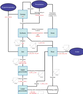
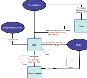
In a first model setup (Model 1, Fig. 3) all processes are reliant on different flow connections. The incoming precipi-tation is saved in a snow storage in case the air temperature is below freezing point and rereleased to the surface storage after snowmelt. All other precipitation is split between the canopy or reaches the surface directly, depending on canopy closure. From the surface, the water is either directly routed to the river or enters three serial soil–groundwater layers, which in turn route water to the river as well. In addition, a fixed amount of water is abstracted from the lower ground-water to simulate drinking ground-water extraction, which in turn is routed to the river. The river then routes all water to the outlet. Thus, it contains the implementations of processes for evapotranspiration, a canopy, snow, surfaces, a river, and upper- and lower groundwater body (Fig. 3).
Following the findings of Singh (2002) all connections in the model with a flow curve (Fig. 3) are described as kine-matic waves (Eq. 1) (Singh, 2002), except for the infiltration and the drinking water abstraction.
Q=Q0 V −V
residual V0
β
, (1)
whereQis the ratio of transferred water,Vresidual(m3) is the volume of water remaining in the storage,V0(m3) is the ref-erence volume to scale the exponent,V is the current volume of water in the storage (m3), andβis a parameter to shape the response curve [–]. The parameterQ0is the flux in m3day−1, when V−Vresidual
V0 =1.
Water that reaches the surface, i.e., throughfall or snowmelt, is routed into the upper soil as infiltration, with the following limits applied:
– Infiltration excess expressed by a maximum surface per-meabilityKsat.
– Saturation excess expressed by a limiting factor calcu-lated from the water content of the first subsurface water storage using a sigmoidal function.
Drinking water abstraction is implemented as a fixed amount of water. As the influence of the drinking water ab-straction is not known, the amount of water abstracted is cal-ibrated. It is transferred to the drinking water storage as long
as the amount of water in the groundwater storage is above a threshold. As this threshold is not exactly known, we in-cluded it as a parameter for calibration. From the drinking water storage, all water abstracted for a given day is routed to the river.
Snowmelt uses a simple degree-day method (see API in CMF, 2017). The snowmelt temperature parameter was cal-ibrated. Interception from the canopy is realized as Rutter interception (Rutter and Morton, 1977). Potential evapotran-spiration was calculated with the modified Hargreaves equa-tion by Samani (2000).
The devised model was tested by using fluxogram graphs. Fluxograms allow creating animated graphs that resemble model structures with all their storages and fluxes and they were used to analyze the implemented model processes (for more information about the fluxogram graph see Jehn, 2018). The size of the storages and fluxes change for each time step according to the amount of water stored or moved. For the fluxogram animations, we used the model with the highest logarithmic Nash–Sutcliffe efficiency (logNSE).
2.4 Incremental model breakdown
To test the influence of different structure elements in Model 1, we used the concept of a one-at-a-time sensitivity analysis, i.e., disabling one process after the other, to track changes (Fig. 4). This resulted in 13 additional models with varying disabled processes (Table 1). In a second step, we disabled up to four processes, to scrutinize the interplay of processes, as proposed by Clark et al. (2011). When a pro-cess was removed, the connections leading to it were then connected to the next nearby storage. For example, if the sur-face storage was removed, the canopy and the snow storage were connected to the soil. Or if the river was removed, all connections leading to it were directly connected to the out-let.
remov-F. U. Jehn et al.: Incremental model breakdown to assess the multi-hypotheses problem 4569
Figure 3.Structure of the Model 1 with water storages (light blue), boundaries (dark blue), temporary storages (white), calibrated parameters (red), fluxes (black arrows) and flow curves (for all applicable fluxes). Water reaching the outlet is shifted 1 day into the future.
ing the irrelevant subprocesses. The code for the models can be found at GitHub (Jehn, 2017). The fluxes in the models were visualized with the fluxogram package (Jehn, 2018). 2.5 Calibration and validation
A model run was separated into a warm-up period of 1 year (1979), a calibration period of 6 years (1980–1985) and a validation period of 3 years (1986–1988). First CMF model runs showed that many simulated discharge peaks occurred 1 day ahead compared to observed data. This is caused by rainfall occurring in the later time of a day, which leads to a reaction in the hydrograph of the following day as water needs time to reach the gauging station (Ficchì et al., 2016). The model, however, reacts directly to this as its input data are resolved in a 24 h time step. Therefore, we shifted the simulated time series 1 day into the future as proposed by Bosch et al. (2004). This led to better calibration results. This
was not needed for HBV Light, in which the MAXBAS pa-rameter accounts for shifting peak discharge.
Figure 4.Flow chart for the method of incremental model breakdown.
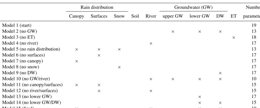
Table 1.Structural elements of the models and amount of parameters. GW is groundwater, DW is drinking water and ET is evapotranspiration. Light gray indicates active components. Dark grey indicates disabled components. The “×” symbol marks the deactivated components.
Rain distribution Groundwater (GW) Number Canopy Surfaces Snow Soil River upper GW lower GW DW ET parameters
Model 1 (start) 19
Model 2 (no GW) × × × 13
Model 3 (no ET) × 18
Model 4 (no river) × 17
Model 5 (no rain distribution) × × × 13
Model 6 (no surfaces) × 17
Model 7 (no canopy) × 17
Model 8 (no snow) × 17
Model 9 (no DW) × 17
Model 10 (no GW/river) × × × × 10
Model 11 (no canopy/surfaces) × × 15
Model 12 (no river/surfaces) × × 15
Model 13 (no lower GW) × 17
Model 14 (no lower GW/DW) × × 15
Model 15 (final) × × × × × 10
was below or above±25 % (optimal value: 0; range:−100 to +∞), and the ratio between the root mean square error and the standard deviation of the measured data (RSR) was < 0.7 (optimal value: 0; range: 0 to∞). As an additional constraint we also included the logarithmic Nash–Sutcliffe efficiency (optimal value: 1; range: 1 to−∞) to allow a better evalu-ation of low flows. The NSE focuses on peak flows and the PBIAS considers the overall model deviation from observed data. It should be noted though that this study does not aim to find the optimal parameter sets for a single model, but to use the knowledge gained from calibration and validation to identify the most important processes in the model structure and use this to improve the model structure and reduce the number of parameters used. The validation period is strictly not used in any selection process to avoid overfitting and only used in the last validation step of the overall method. To fi-nally compare the models that were able to produce behav-ioral runs, we used the median to evaluate the typical be-havior of a run of a given model and the maximal value to determine the best possible performance.
The sampling of the parameter space for calibration was done by Latin hypercube sampling (McKay et al., 1979) implemented via SPOTPY (Houska et al., 2015). All mod-els were run 300 000 times each, using a High-Performance Computing Cluster. See the tutorial section of CMF (2017)
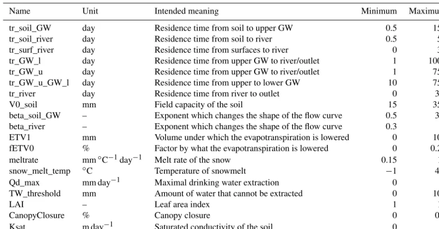
for more detailed information on the coupling of CMF with SPOTPY for model calibration. Implemented param-eter boundaries for Model 1 are given in Table 2 and re-mained fixed for all further-developed model structures to ensure comparability.
The lower and upper bounds for V0_soil and ETV1 were taken from Blume et al. (2016) for typical field capacities re-ported for German soils in the range of 20 to 300. Canopy parameters are in line with values provided by Breuer et al. (2003). Groundwater transit times are roughly corre-sponding with the findings of Wittmann (2002) and Wend-land et al. (2011). For all other parameters, we could not find reliable data and thus estimated them subjectively. The pa-rameters use a wide range intentionally to allow the parame-ters to adapt to the very different model structures.
2.6 Benchmarking model
[image:6.612.53.546.186.391.2]par-F. U. Jehn et al.: Incremental model breakdown to assess the multi-hypotheses problem 4571
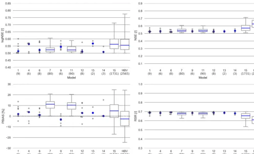
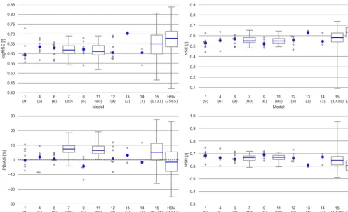
Figure 5.Distribution of the values of the behavioral runs in the calibration period. Plotted as a box plot if the number of behavioral runs is above 10. Number of behavioral runs are in brackets under the name of the model. Blue dot or line marks the median.
simonious model. We used the simplest setup of HBV Light with a single soil storage and no lapse rate. As HBV Light has no internal way to calculate potential evapotranspiration, we used the same approach by Samani (2000) as for all other models.
3 Results
3.1 Behavioral runs of Model 1 to 14
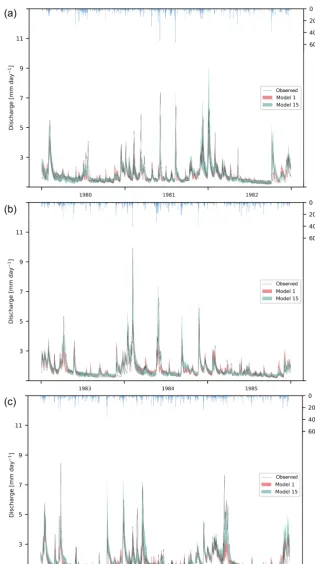
Model 1 was able to achieve nine behavioral runs. The model has a better performance in the validation period (Figs. 5, 6). This is true for all other models as well. The simulated dis-charge is rather erratic (Fig. 7); i.e., it reacts directly on small changes in precipitation. Those quick reactions are timed correctly. However, they overestimate the discharge from small precipitation events, while underestimating large ones. These differences are larger in summer than in winter. This behavior leads to underestimated high flows and many over-estimated small peaks, while the overall simulated amounts are unbiased. Investigation of storages and fluxes (fluxogram graph: https://youtu.be/cP0PfDpfW88, last access: 23 Au-gust 2018) shows that most of the water is stored in the upper groundwater storage, while the lower groundwater storage is removed directly by the drinking water production, as soon
as it is above the threshold. Only very small amounts of wa-ter are stored in the surface storage, the canopy storage and the soil storage. From the soil storage and the canopy storage large amounts of water evaporate, often exceeding the flow to the outlet. The river storage is mostly recharged from the groundwater and the drinking water storage. The soil stor-age contributes significantly to the river storstor-age only at large precipitation events or during snowmelt. Overall, Model 1 slightly overestimates low flows and the evapotranspiration, while largely underestimating the peaks.
Most of the deleted model processes from the most com-plex Model 1 led to more behavioral runs (Figs. 5, 6). Model 1 and 4 (no river storage), 6 (no surface storage), 9 (no drink-ing water simulation), 12 (no river and surface storages), 13 (no lower groundwater storage) and 14 (no groundwater stor-ages and drinking water simulation) have between two to nine behavioral runs. Model 7 (no canopy) and 11 (no canopy and surface storage) are able to produce 80 and 90 behavioral runs respectively (Figs. 5, 6). The remaining models 2 (no groundwater storages), 3 (no evapotranspiration), 5 (no rain distribution), 8 (no snow) and 10 (no groundwater and river storages) were not able to produce behavioral runs.
Table 2.Lower and upper parameters bounds of all models and their indented meaning. GW is groundwater.
Name Unit Intended meaning Minimum Maximum tr_soil_GW day Residence time from soil to upper GW 0.5 150 tr_soil_river day Residence time from soil to river 0.5 55 tr_surf_river day Residence time from surfaces to river 0 30 tr_GW_l day Residence time from upper GW to river/outlet 1 1000 tr_GW_u day Residence time from upper GW to river/outlet 1 750 tr_GW_u_GW_l day Residence time from upper to lower GW 10 750 tr_river day Residence time from river to outlet 0 3.5 V0_soil mm Field capacity of the soil 15 350 beta_soil_GW – Exponent which changes the shape of the flow curve 0.5 3.2 beta_river – Exponent which changes the shape of the flow curve 0.3 4 ETV1 mm Volume under which the evapotranspiration is lowered 0 100 fETV0 % Factor by what the evapotranspiration is lowered 0 0.25 meltrate mm◦C−1day−1 Melt rate of the snow 0.15 10 snow_melt_temp ◦C Temperature of snowmelt −1 4.2 Qd_max mm day−1 Maximal drinking water extraction 0 3 TW_threshold mm Amount of water that cannot be extracted 0 100
LAI – Leaf area index 1 12
CanopyClosure % Canopy closure 0 0.5 Ksat m day−1 Saturated conductivity of the soil 0 1
1, while Model 1 has a PBIAS better than the other mod-els. Particularly for Model 13 (no lower groundwater stor-age), the median values for the objective functions outper-form Model 1.
3.2 Construction and behavioral runs of Model 15 We can report that representation of model processes for the upper groundwater body, evapotranspiration and snow has a positive impact on model performance in the Fulda catchment, given the increased median values of the objec-tive functions (Figs. 5, 6), as when those processes are ex-cluded the models struggle to produce behavioral runs. The exclusion of the canopy and drinking water have a more or less neutral impact on the median performance of the behav-ioral runs (Figs. 5, 6), whereas the chosen implementations of the river, the surfaces and the lower groundwater affect the model quality negatively (Figs. 5, 6). The structure of Model 15 was created after all the other models had been evaluated. For this, we used the process knowledge gained from the reduced models (see discussion) and constructed Model 15 with only those processes which had proven to have a positive impact on the quality of the results. There-fore, Model 15 consists only of those processes most impor-tant for the given Fulda catchment (Fig. 9). In comparison with the model structure of Model 1, the processes surface water storage, lower groundwater storage, drinking water ex-traction, river storage and the simulation of the canopy were disabled.
Profiting from the insights of the models with disabled processes, Model 15 performs better than Model 1. The RSR, NSE and the logNSE depict better values, both in the
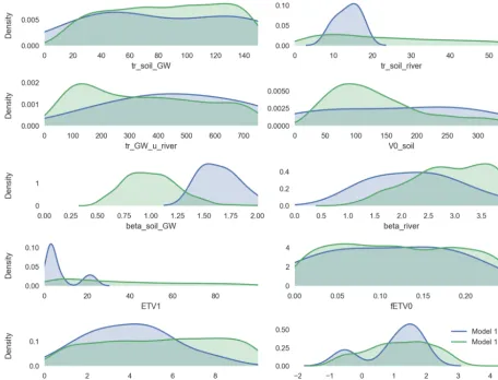
valida-tion and calibravalida-tion period, while the PBIAS is slightly worse for both cases (Figs. 5, 6). In particular, the maximal values for the logNSE, NSE and RSR are much better than Model 1. As for all other models, the performance increases from the calibration to the validation period for Model 15. The simu-lated hydrograph is a lot less erratic than the one from Model 1 (Fig. 7). In addition, the peaks fit better than in Model 1. However, summer peaks are less likely to be predicted than those during the rest of the year (Fig. 7). The overestima-tion of low flow in Model 1 is apparent on fewer days. In addition to this increase in the performance in comparison with Model 1, Model 15 uses nine parameters less (Table 1). The remaining 10 parameters in Model 15 behave differently from the same ones in Model 1 (Fig. 8). Some parameters like tr_soil_GW and fEVT0 have almost the same density distribution. Nevertheless, there are several parameters like tr_soil_river and ETV1 whose density is much more focused around a specific value for Model 1 than for Model 15. 3.3 Behavioral runs of HBV Light
F. U. Jehn et al.: Incremental model breakdown to assess the multi-hypotheses problem 4573
Figure 6.Distribution of the values of the behavioral runs in the validation period. Plotted as a box plot if the number of behavioral runs is above 10. Number of behavioral runs are in brackets under the name of the model. Blue dot or line marks the median.
the values of the objective functions in the validation period, hinting to a large parameter equifinality.
4 Discussion 4.1 Overview
The results show that Model 1 fell short on simulating the catchment correctly, mainly caused by a slow reaction to pre-cipitation events, which reduced discharge peak prediction and caused the model to focus on evapotranspiration to han-dle the excess water. Nevertheless, it was a good basis to de-termine relevant processes by incremental model breakdown. Insights from this led to an improvement in the performance of Model 15, while at the same time allowing a reduction of the number of parameters (from n=19 to n=10) (Ta-ble 1). Nevertheless, even this improvement did not allow Model 15 to outperform HBV Light. Nevertheless, this sug-gests that the method of incremental model breakdown is a good way to improve model performance and reduce equifi-nality through parameter reduction, which improves the iden-tifiability of the model structure (Ambroise, 2004). It enables insight into which processes are important for discharge sim-ulations in a given catchment. It also allows revealing errors, using them “as a means of discovery” of false model
assump-tions (Elliott, 2004). It should be noted that this method does not necessarily lead to an improved model performance, but it allows creating a model which relies on fewer processes, parameters and assumptions, thus being an application of Oc-cam’s razor (Clark et al., 2011).
4.2 Inspection of internal processes
F. U. Jehn et al.: Incremental model breakdown to assess the multi-hypotheses problem 4575
Figure 8.Distribution of all parameters shared by Model 1 (blue) and Model 15 (green), fitted with kernel density.
the rather low population of 159 persons per km2in the re-gion, and neither water withdrawal for irrigation nor water-consuming industries are relevant players in the region’s wa-ter cycle. The canopy, however, is commonly regarded as an important factor, as interception can cause more than 25 % of the rainfall not to reach the ground (Link et al., 2004). However, Model 15 was able to get better values for the ob-jective functions than Model 1 even though the canopy was disabled (Figs. 5, 6). Seibert and Vis (2012) showed before that canopy storages are not very important for humid cli-mates, as in our case. However, Fenicia et al. (2008) found that this is not the case for dry environments. This can be seen as an example on how incremental model breakdown pro-duces models that are adopted to the environment of model testing. Also, the current implementation of the canopy as-sumes a fixed canopy storage for the whole year. A more realistic approach should be implemented for future appli-cations, as was for example realized in the plot-scale CMF application coupled to plant growth models for winter wheat (Houska et al., 2014) and perennial grassland (Kellner et al., 2017).
The river storage is most likely too small to be an im-portant reservoir in comparison to the catchment. The sur-face storages probably do not contribute to the runoff itself, because the catchment is mostly vegetated, which impedes overland flow. Lower groundwater was included because of the ability of the sand- and limestone in the catchment to store large quantities of water and because of the tritium-based tracer experiments of Wittmann (2002). He found two distinct groundwater aquifers in the catchment. Their study comes to the results that the lowest of the aquifers is very large. However, our posterior parameter boundaries indicate a very slow response.
Figure 9.Structure of the final Model 15 with water storages (light blue), boundaries (dark blue), temporary storages (white), calibrated parameters (red), fluxes (black arrows) and flow curves (for all applicable fluxes). Water reaching the outlet is shifted 1 day into the future.
is that the snowmelt occurs evenly distributed over the whole catchment, so that the complete snowmelt in the model takes only a few days, often even only 1 day. It might also be linked to the evapotranspiration. In times of low evapotranspiration, the water is forced to leave the model as discharge. There-fore, large precipitation events are directly transferred to large peaks. During times of high evapotranspiration, much water can be released into the atmosphere, and as the water in the soil storage of Model 15 flows proportionately more of the storage is already high; this allows the water to stay longer in the soil, which in turn allows more evapotranspira-tion.
The fluxograms showed that Model 1 did not use the drinking water storage and used the canopy storage only rarely. These observations underline the demand of Clark et al. (2011) that the internal procedures of a hydrological model should be inspected as well, to better understand its functioning. The fluxograms helped to detect that canopy and drinking water are not used by the model.
When examining the median model performance of all re-duced models and the resulting Model 15, one can see that the median values of the objective functions of Model 15 are similar to those of Model 13 (Figs. 5, 6). Model 15 is considered to be the better representation of the catchment compared to Model 13, as it has a more streamlined structure and seven parameters less. In addition, the good values for Model 13 are mainly caused by the low number of
behav-ioral runs (n=2), allowing one very good run to distort the results. Also, Model 15 reaches higher maximal values for the objective functions.
This improved performance of Model 15 in comparison with Model 1 is overshadowed though, by the higher equifi-nality of some parameters in Model 15 (Fig. 8). In Model 1 for example the parameter EVT1 has two very distinct peaks, while the Model 15 distribution for this parameter is spread out widely. The behavior of ETV1 might also be linked to the rightward shift of the parameter beta_soil_GW. This pa-rameter controls the speed in which water leaves the soil in the direction of the groundwater. The increase in its value lets the water stay longer in the soil storage, allowing more evapotranspiration, which in turn allows the parameter ETV1 to be handled more flexible by the model. This might indi-cate that the parameters of Model 15 need to compensate for the simpler model structure in comparison with Model 1, by having a wider range of possible values. This would allow a single parameter to express the behavior of several processes at once.
4.3 Comparison with HBV Light
F. U. Jehn et al.: Incremental model breakdown to assess the multi-hypotheses problem 4577
shape of the hydrograph in general. Model 1 seems to be able to get the shape of the hydrograph during low flow correct (Fig. 7), while HBV excels at simulating the peaks. Model 15 is somewhere in between. Those differences are probably caused by the number of storages in the models and processes that mimic saturation excess.
Model 15 and HBV Light are quite similar with regard to their model structure and the considered hydrological pro-cesses. The main differences in model performances are the way the mathematical process descriptions are implemented. HBV Light has a maximal value for percolation and the trian-gular weighting function that changes the shape of the flow curve (Seibert and Vis, 2012) .With the maximal value for percolation, additional water is forced to become discharge, as there is no other way it could go. This allows HBV Light to forecast the peaks better but also might make the model react too quickly. This behavior though is counteracted by the tri-angular weighting function of HBV Light. In contrast, Model 15 predicts the peaks correctly only during times of low evap-otranspiration. Another main difference exists for the simu-lation of base flow. Model 1 depicts a highly correlated base flow to the observed one, but the model is overestimating the total amount. Model 15 and HBV Light mimic the shape and timing of the low flow worse, but predict the amounts better. One reasons for this behavior might be that a model needs a good representation of the groundwater to simulate discharge minima (Plesca et al., 2012), which is the case for Model 1, but only to a lesser extent for HBV Light and Model 15. Those findings highlight the problems occurring when a complex model is reduced in its complexity. Therefore, even if the simpler models are able to get higher values for the objective functions they seem to lose some other traits (like the ability to predict the correct shape of the low flow in this case) in an unpredictable manner.
4.4 Does model incremental breakdown allow the construction of improved models?
The improved performance of Model 15 shows that a pri-ori model selection can raise problems, as the models with different process implementations deliver very different re-sults. Those differences cannot be explored if only one pre-defined model is used. This is in line with the findings of Ley et al. (2016), who used predefined model structures on a large amount of different catchments and found that no model was able to simulate all catchments well. Similar re-sults were also found by Kavetski and Fenicia (2011) and Fenicia et al. (2014), who showed that lumped models need to be tailored for single catchments as they are often over-simplified. Therefore, starting from a complex model, sim-plifying it only where justified, could help resolve the issue of oversimplifications in lumped models.
Lumped models have the advantage of an easy setup and low data requirements, but this comes at the cost of not be-ing able to address the spatial heterogeneity of the catch-ments (Ley et al., 2016) and that the parameters and struc-tures have no direct equivalence in the real world (Bergström and Graham, 1998). Therefore, a lumped model structure might simply have been too simple for the upper section of the Fulda catchment, calling for a semi-distributed or even distributed model setup. This is also hinted by a study by Fink and Koch (2010), who where able to model the Fulda catchment quite well with a modified semi-distributed ver-sion of SWAT. Overall, we think that the proposed method of incremental model breakdown led to an improvement in model performance. In addition, the model complexity and amount of parameters with this equifinality were reduced. In this regard, the incremental model breakdown is different to methods like sensitivity analysis where the model structure is untouched, as we reduce the structural model complexity. Both topics are often stated as the main goals of model de-velopment, e.g., Efstratiadis and Koutsoyiannis (2010) and Gupta and Nearing (2014).
Incremental model breakdown bears, as any model in-tercomparison study of calibrated models, a risk of overfit-ting. In the context of this study, overfitting would results in the acceptance of a process that seems only by chance relevant in the calibration period but has only weak predic-tive power. Another overfitting effect would be a preference of parameter-rich models. An indicator for overfitting is the great results in the calibration period but flawed results dur-ing validation. This shows the importance of a validation pe-riod that is never used in any selection process, neither for structure nor for parameters. In this study, the performance of the models during validation generally exceeded the per-formance of the calibration period, despite the different char-acteristics of those periods. For future studies, longer data time series should be split into three independent periods: (1) parameter calibration period, (2) model selection period and (3) the a posteriori selection process validation period. A second effect when both structural and parameter uncertainty are to be compared, we are not only facing an equifinality of parameter sets but an equifinality of structures. We based the recognition of relevant processes on the rejection and not the optimization of certain model structures, as suggested by Beven (2006) to gain a robust method. All in all, incremental model breakdown and inspection of parameter distribution, as well as comparison with already established models and the flow path in a model with a fluxogram, might help deter-mine if models do the right things for the right reasons.
5 Conclusion
hydrological processes in a model and the reconstruction of the starting model structure to a more efficient version. We conclude that the method provided offers a useful ap-proach in the identification of relevant hydrological pro-cesses. Model frameworks such as CMF facilitate the devel-opment of such an approach.
We acknowledge that this study might have led to different results if a different time step had been used. However, this does not impair the use of the method of incremental model breakdown, as it is meant to find the most important pro-cess in a given model setup and we assume that this mainly depends on the way the model is constructed and not nec-essarily on the temporal resolution of the input data, at least for the catchment size we investigated in this study. Never-theless, we recognize that this is a potential direction for fu-ture research. Sikorska and Seibert (2018) recently showed that data of sub-daily resolution become relevant to achieve acceptable model performances with decreasing catchment sizes of 200 km2and smaller.
The incremental model breakdown can be used best in two cases: (1) finding out why an existing good model does pro-duce good results in the sense of a diagnostic tool to assess model structures; or, as in this study, (2) determining which processes are most relevant, to allow the streamlining of a model.
One goal of this study was to find another strategic way to test the multiple implementations of catchment functioning. We were able to distinguish between unnecessary and rele-vant model processes. Further, it became clearer what causes those problems, by examining the model piece by piece as proposed by Clark et al. (2016). Therefore, this method can be seen as a useful third way, in addition to stepwise model building (Bai et al., 2009; Westerberg and Birkel, 2015) and the comparison of predefined structures (van Esse et al., 2013; Kavetski and Fenicia, 2011), to explore the realm of multiple hypotheses and help to keep an open mind, which is needed when going from a complex model to a simpler one. (Bergström, 1991). We propose future research should consider an automatic assemblage of model structures to test not only a manually manageable number of models but rather scan a larger variety of feasible combinations, which in turn would allow a completely exhaustive exploration of the space of possible model structure.
Data availability. Datasets are available by contacting the Hes-sian Agency for Nature Conservation, Environment and Ge-ology (HLNUG) (https://www.hlnug.de/service/english.html, last access: 23 August 2018). The code for all model structures (https://doi.org/10.5281/zenodo.1067939; Jehn, 2017) and the flux-ogram (https://doi.org/10.5281/zenodo.1137703; Jehn, 2018) can be found at GitHub by following the links in the citations.
Author contributions. FUJ, LB and PK conceived and designed the study. PK acquired the forcing data. FUJ built the models and an-alyzed the results of the model runs. All authors aided in the in-terpretation and discussion of the results and the writing of the manuscript.
Competing interests. The authors declare that they have no conflict of interest.
Acknowledgements. We thank the Hessisches Landesamt für Naturschutz, Umwelt und Geologie for providing the meteorolog-ical and discharge data as well as Albrecht Weerts, Lieke Melsen, François Anctil and one anonymous referee for their valuable comments which allowed us to improve this paper substantially. Edited by: Albrecht Weerts
Reviewed by: Lieke Melsen, François Anctil, and one anonymous referee
References
Ambroise, B.: Variable “active” versus “contributing” areas or pe-riods: a necessary distinction, Hydrol. Process., 18, 1149–1155, https://doi.org/10.1002/hyp.5536, 2004.
Bai, Y., Wagener, T., and Reed, P.: A top-down frame-work for watershed model evaluation and selection un-der uncertainty, Environ. Modell. Softw., 24, 901–916, https://doi.org/10.1016/j.envsoft.2008.12.012, 2009.
Bergström, S.: Principles and Confidence in Hy-drological Modelling, Hydrol. Res., 22, 123–136, https://doi.org/10.2166/nh.1991.0009, 1991.
Bergström, S. and Graham, L. P.: On the scale problem in hydrological modelling, J. Hydrol., 211, 253–265, https://doi.org/10.1016/S0022-1694(98)00248-0, 1998. Beven, K.: Towards integrated environmental models of
every-where: uncertainty, data and modelling as a learning process, Hy-drol. Earth Syst. Sci., 11, 460–467, https://doi.org/10.5194/hess-11-460-2007, 2007.
Beven, K. and Binley, A.: The future of distributed models: Model calibration and uncertainty prediction, Hydrol. Process., 6, 279– 298, https://doi.org/10.1002/hyp.3360060305, 1992.
Beven, K. J.: Uniqueness of place and process representations in hydrological modelling, Hydrol. Earth Syst. Sci., 4, 203–213, https://doi.org/10.5194/hess-4-203-2000, 2000.
Beven, K. J.: On hypothesis testing in hydrology, Hydrol. Process., 15, 1655–1657, https://doi.org/10.1002/hyp.436, 2001.
Beven, K. J.: Towards an alternative blueprint for a physically based digitally simulated hydrologic response modelling system, Hydrol. Process., 16, 189–206, https://doi.org/10.1002/hyp.343, 2002.
Beven, K. J.: A manifesto for the equifinality thesis, J. Hydrol., 320, 18–36, https://doi.org/10.1016/j.jhydrol.2005.07.007, 2006. Beven, K. J.: Facets of uncertainty: epistemic
F. U. Jehn et al.: Incremental model breakdown to assess the multi-hypotheses problem 4579
Beven, K. J. and Kirkby, M. J.: A physically based, vari-able contributing area model of basin hydrology/Un modèle à base physique de zone d’appel variable de l’hydrologie du bassin versant, Hydrol. Sci. B., 24, 43–69, https://doi.org/10.1080/02626667909491834, 1979.
Blume, H.-P., Brümmer, G. W., Horn, R., Kandeler, E., Kögel-Knabner, I., Kretzschmar, R., Stahr, K., Wilke, B.-M., Scheffer, F., and Schachtschabel, P.: Scheffer/Schachtschabel Lehrbuch der Bodenkunde, 16. Auflage, (Nachdruck), Springer Spektrum, Berlin, Heidelberg, 2016.
Bosch, D. D., Sheridan, J. M., Batten, H. L., and Arnold, J. G.: Evaluation of the SWAT model on a coastal plain agricultural watershed, T. ASAE, 47, 1493–1506, https://doi.org/10.13031/2013.17629, 2004.
Breuer, L., Eckhardt, K., and Frede, H.-G.: Plant parameter values for models in temperate climates, Ecol. Model., 169, 237–293, https://doi.org/10.1016/S0304-3800(03)00274-6, 2003. Breuer, L., Huisman, J. A., Willems, P., Bormann, H., Bronstert,
A., Croke, B. F. W., Frede, H.-G., Gräff, T., Hubrechts, L., Jakeman, A. J., Kite, G., Lanini, J., Leavesley, G., Lettenmaier, D. P., Lindström, G., Seibert, J., Sivapalan, M., and Viney, N. R.: Assessing the impact of land use change on hydrol-ogy by ensemble modeling (LUCHEM). I: Model intercompar-ison with current land use, Adv. Water Resour., 32, 129–146, https://doi.org/10.1016/j.advwatres.2008.10.003, 2009. Buytaert, W., Reusser, D., Krause, S., and Renaud, J.-P.: Why can’t
we do better than Topmodel?, Hydrol. Process., 22, 4175–4179, https://doi.org/10.1002/hyp.7125, 2008.
Clark, M. P. and Kavetski, D.: Ancient numerical daemons of conceptual hydrological modeling: 1. Fidelity and effi-ciency of time stepping schemes: Numerical daemons of hy-drological modeling, 1, Water Resour. Res., 46, W10510, https://doi.org/10.1029/2009WR008894, 2010.
Clark, M. P., Kavetski, D., and Fenicia, F.: Pursuing the method of multiple working hypotheses for hydrological modeling: Hy-pothesis testing in hydrology, Water Resour. Res., 47, W09301, https://doi.org/10.1029/2010WR009827, 2011.
Clark, M. P., Nijssen, B., Lundquist, J. D., Kavetski, D., Rupp, D. E., Woods, R. A., Freer, J. E., Gutmann, E. D., Wood, A. W., Brekke, L. D., Arnold, J. R., Gochis, D. J., and Rasmussen, R. M.: A unified approach for process-based hydrologic mod-eling: 1. Modeling concept: A unified approach for process-based hydrologic modeling, Water Resour. Res., 51, 2498–2514, https://doi.org/10.1002/2015WR017198, 2015a.
Clark, M. P., Nijssen, B., Lundquist, J. D., Kavetski, D., Rupp, D. E., Woods, R. A., Freer, J. E., Gutmann, E. D., Wood, A. W., Gochis, D. J., Rasmussen, R. M., Tarboton, D. G., Ma-hat, V., Flerchinger, G. N., and Marks, D. G.: A unified ap-proach for process-based hydrologic modeling: 2. Model im-plementation and case studies: A unified approach for process-based hydrologic modeling, Water Resour. Res., 51, 2515–2542, https://doi.org/10.1002/2015WR017200, 2015b.
Clark, M. P., Schaefli, B., Schymanski, S. J., Samaniego, L., Luce, C. H., Jackson, B. M., Freer, J. E., Arnold, J. R., Moore, R. D., Istanbulluoglu, E., and Ceola, S.: Improving the theoretical un-derpinnings of process-based hydrologic models: Narrowing the gap between hydrologic theory and models, Water Resour. Res., 52, 2350–2365, https://doi.org/10.1002/2015WR017910, 2016.
CMF: Catchment Modelling Framework Website, available at: http: //fb09-pasig.umwelt.uni-giessen.de/cmf, last access: 12 Febru-ary 2017.
Djabelkhir, K., Lauvernet, C., Kraft, P., and Carluer, N.: Development of a dual permeability model within a hydrological catchment modeling framework: 1D application, Sci. Total Environ., 575, 1429–1437, https://doi.org/10.1016/j.scitotenv.2016.10.012, 2017.
Efstratiadis, A. and Koutsoyiannis, D.: One decade of multi-objective calibration approaches in hydrologi-cal modelling: a review, Hydrolog. Sci. J., 55, 58–78, https://doi.org/10.1080/02626660903526292, 2010.
Elliott, K.: Error as Means to Discovery, Philos. Sci., 71, 174–197, https://doi.org/10.1086/383010, 2004.
Fenicia, F., Savenije, H. H. G., Matgen, P., and Pfister, L.: Understanding catchment behavior through stepwise model concept improvement, Water Resour. Res., 44, W01402, https://doi.org/10.1029/2006WR005563, 2008.
Fenicia, F., Kavetski, D., and Savenije, H. H. G.: Elements of a flexible approach for conceptual hydrological modeling: 1. Mo-tivation and theoretical development: Flexible framework for hydrological modeling, 1, Water Resour. Res., 47, W11510, https://doi.org/10.1029/2010WR010174, 2011.
Fenicia, F., Kavetski, D., Savenije, H. H. G., Clark, M. P., Schoups, G., Pfister, L., and Freer, J.: Catchment properties, function, and conceptual model representation: is there a correspondence?, Hy-drol. Process., 28, 2451–2467, https://doi.org/10.1002/hyp.9726, 2014.
Ficchì, A., Perrin, C., and Andréassian, V.: Impact of temporal resolution of inputs on hydrological model performance: An analysis based on 2400 flood events, J. Hydrol., 538, 454–470, https://doi.org/10.1016/j.jhydrol.2016.04.016, 2016.
Fink, G. S. M. and Koch, M.: Climate change effects on the wa-ter balance in the Fulda catchment, Germany, during the 21st centruy, conference paper at Symposium on sustainable wa-ter ressource management and climate change adaption, Nakon Pathom., 2010.
Gharari, S., Hrachowitz, M., Fenicia, F., Gao, H., and Savenije, H. H. G.: Using expert knowledge to increase realism in environmental system models can dramatically reduce the need for calibration, Hydrol. Earth Syst. Sci., 18, 4839–4859, https://doi.org/10.5194/hess-18-4839-2014, 2014.
Gupta, H. V. and Nearing, G. S.: Debates-the future of hydrolog-ical sciences: A (common) path forward? Using models and data to learn: A systems theoretic perspective on the future of hydrological science, Water Resour. Res., 50, 5351–5359, https://doi.org/10.1002/2013WR015096, 2014.
Haas, E., Klatt, S., Fröhlich, A., Kraft, P., Werner, C., Kiese, R., Grote, R., Breuer, L., and Butterbach-Bahl, K.: LandscapeD-NDC: a process model for simulation of biosphere–atmosphere– hydrosphere exchange processes at site and regional scale, Land-scape Ecol., 28, 615–636, https://doi.org/10.1007/s10980-012-9772-x, 2013.
Hindmarsh, A. C., Brown, P., Grant, K. E., Lee, S. L., Serban, R., Shumaker, D. E., and Woodward, C. S.: SUNDIALS: Suite of nonlinear and differential/algebraic equation solvers, ACM T. Math. Software, 31, 363–396, 2005.
Stamm, C., Stoll, S., Blöschl, G., and Flühler, H.: Comparative predictions of discharge from an artificial catchment (Chicken Creek) using sparse data, Hydrol. Earth Syst. Sci., 13, 2069– 2094, https://doi.org/10.5194/hess-13-2069-2009, 2009. Houska, T., Multsch, S., Kraft, P., Frede, H.-G., and Breuer, L.:
Monte Carlo-based calibration and uncertainty analysis of a cou-pled plant growth and hydrological model, Biogeosciences, 11, 2069–2082, https://doi.org/10.5194/bg-11-2069-2014, 2014. Houska, T., Kraft, P., Chamorro-Chavez, A., and Breuer,
L.: SPOTting Model Parameters Using a Ready-Made Python Package, PLOS ONE, 10, e0145180, https://doi.org/10.1371/journal.pone.0145180, 2015.
Houska, T., Kraft, P., Liebermann, R., Klatt, S., Kraus, D., Haas, E., Santabarbara, I., Kiese, R., Butterbach-Bahl, K., Müller, C., and Breuer, L.: Rejecting hydro-biogeochemical model struc-tures by multi-criteria evaluation, Environ. Modell. Softw., 93, 1–12, https://doi.org/10.1016/j.envsoft.2017.03.005, 2017. Hublart, P., Ruelland, D., Dezetter, A., and Jourde, H.: Reducing
structural uncertainty in conceptual hydrological modelling in the semi-arid Andes, Hydrol. Earth Syst. Sci., 19, 2295–2314, https://doi.org/10.5194/hess-19-2295-2015, 2015.
Hudson, G. and Wackernagel, H.: Mapping temperature using krig-ing with external drift: Theory and an example from scotland, Int. J. Climatol., 14, 77–91, https://doi.org/10.1002/joc.3370140107, 1994.
Jehn, F.: Zutn/Incremental_Breakdown: Reupload, https://doi.org/10.5281/zenodo.1067939, 2017.
Jehn, F.: Zutn/Fluxogram: First Public Version Of The Fluxogram, https://doi.org/10.5281/zenodo.1137703, 2018.
Kavetski, D. and Clark, M. P.: Numerical troubles in con-ceptual hydrology: Approximations, absurdities and im-pact on hypothesis testing, Hydrol. Process., 25, 661–670, https://doi.org/10.1002/hyp.7899, 2011.
Kavetski, D. and Fenicia, F.: Elements of a flexible ap-proach for conceptual hydrological modeling: 2. Applica-tion and experimental insights: Flexible framework for hy-drological modeling, 2, Water Resour. Res., 47, W11511, https://doi.org/10.1029/2011WR010748, 2011.
Kavetski, D., Fenicia, F., and Clark, M. P.: Impact of tempo-ral data resolution on parameter inference and model iden-tification in conceptual hydrological modeling: Insights from an experimental catchment, Water Resour. Res., 47, W05501, https://doi.org/10.1029/2010WR009525, 2011.
Kellner, J., Multsch, S., Houska, T., Kraft, P., Müller, C., and Breuer, L.: A coupled hydrological-plant growth model for simulating the effect of elevated CO 2 on a temperate grassland, Agr. Forest Meteorol., 246, 42–50, https://doi.org/10.1016/j.agrformet.2017.05.017, 2017.
Kraft, P., Multsch, S., Vaché, K. B., Frede, H.-G., and Breuer, L.: Using Python as a coupling platform for integrated catchment models, Adv. Geosci., 27, 51–56, https://doi.org/10.5194/adgeo-27-51-2010, 2010.
Kraft, P., Vaché, K. B., Frede, H.-G., and Breuer, L.: CMF: A Hydrological Programming Language Extension For Inte-grated Catchment Models, Environ. Modell. Softw., 26, 828– 830, https://doi.org/10.1016/j.envsoft.2010.12.009, 2011. Ley, R., Hellebrand, H., Casper, M., and Fenicia, F.: Is Catchment
Classification Possible by Means of Multiple Model Structures?
A Case Study Based on 99 Catchments in Germany, Hydrology, 3, 22, https://doi.org/10.3390/hydrology3020022, 2016. Link, T. E., Unsworth, M., and Marks, D.: The
dy-namics of rainfall interception by a seasonal temper-ate rainforest, Agr. Forest Meteorol., 124, 171–191, https://doi.org/10.1016/j.agrformet.2004.01.010, 2004.
Maier, N., Breuer, L., and Kraft, P.: Prediction and uncer-tainty analysis of a parsimonious floodplain surface water-groundwater interaction model, Water Resour. Res., 53 , 7678– 7695, https://doi.org/10.1002/2017WR020749, 2017.
McKay, M. D., Beckman, R. J., and Conover, W. J.: A Comparison of Three Methods for Selecting Values of Input Variables in the Analysis of Output from a Computer Code, Technometrics, 21, 239–245, https://doi.org/10.2307/1268522, 1979.
Moriasi, D. N., Arnold, J. G., Liew, M. W. V., Bingner, R. L., Harmel, R. D., and Veith, T. L.: Model Eval-uation Guidelines for Systematic Quantification of Accu-racy in Watershed Simulations, T. ASABE, 50, 885–900, https://doi.org/10.13031/2013.23153, 2007.
Orlowski, N., Kraft, P., Pferdmenges, J., and Breuer, L.: Exploring water cycle dynamics by sampling multiple stable water isotope pools in a developed landscape in Germany, Hydrol. Earth Syst. Sci., 20, 3873–3894, https://doi.org/10.5194/hess-20-3873-2016, 2016.
Plesca, I., Timbe, E., Exbrayat, J.-F., Windhorst, D., Kraft, P., Cre-spo, P., Vaché, K. B., Frede, H.-G., and Breuer, L.: Model in-tercomparison to explore catchment functioning: Results from a remote montane tropical rainforest, Ecol. Model., 239, 3–13, https://doi.org/10.1016/j.ecolmodel.2011.05.005, 2012. Rawlins, M. A., Willmott, C. J., Shiklomanov, A., Linder, E.,
Frol-king, S., Lammers, R. B., and Vörösmarty, C. J.: Evaluation of trends in derived snowfall and rainfall across Eurasia and link-ages with discharge to the Arctic Ocean, Geophys. Res. Lett., 33, L07403, https://doi.org/10.1029/2005GL025231, 2006. Rhönenergie Fulda GmbH: Trinkwassergewinnung im Fulda
Einzugsgebiet, available at: https://re-fd.de/trinkwasser/ der-weg-des-trinkwassers, last access: 12 January 2017. Ritter, A. and Muñoz-Carpena, R.: Performance evaluation of
hy-drological models: Statistical significance for reducing subjec-tivity in goodness-of-fit assessments, J. Hydrol., 480, 33–45, https://doi.org/10.1016/j.jhydrol.2012.12.004, 2013.
Rutter, A. J. and Morton, A. J.: A Predictive Model of Rainfall Inter-ception in Forests. III. Sensitivity of The Model to Stand Param-eters and Meteorological Variables, J. Appl. Ecol., 14, 567–588, https://doi.org/10.2307/2402568, 1977.
Samani, Z.: Estimating solar radiation and evapotranspiration using minimum climatological data, J. Irrig. Drain. Eng., 126, 265– 267, 2000.
Seibert, J. and Vis, M. J. P.: Teaching hydrological modeling with a user-friendly catchment-runoff-model software package, Hydrol. Earth Syst. Sci., 16, 3315–3325, https://doi.org/10.5194/hess-16-3315-2012, 2012.
Sikorska, A. E. and Seibert, J.: Appropriate temporal res-olution of precipitation data for discharge modelling in pre-alpine catchments, Hydrolog. Sci. J., 63, 1–16, https://doi.org/10.1080/02626667.2017.1410279, 2018. Singh, V. P.: Is hydrology kinematic?, Hydrol. Process., 16, 667–
F. U. Jehn et al.: Incremental model breakdown to assess the multi-hypotheses problem 4581
Son, K. and Sivapalan, M.: Improving model structure and re-ducing parameter uncertainty in conceptual water balance mod-els through the use of auxiliary data: Improving model struc-ture through auxiliary data, Water Resour. Res., 43, W01415, https://doi.org/10.1029/2006WR005032, 2007.
Todini, E.: Hydrological catchment modelling: past, present and future, Hydrol. Earth Syst. Sci., 11, 468–482, https://doi.org/10.5194/hess-11-468-2007, 2007.
van Esse, W. R., Perrin, C., Booij, M. J., Augustijn, D. C. M., Feni-cia, F., Kavetski, D., and Lobligeois, F.: The influence of concep-tual model structure on model performance: a comparative study for 237 French catchments, Hydrol. Earth Syst. Sci., 17, 4227– 4239, https://doi.org/10.5194/hess-17-4227-2013, 2013. Wendland, F., Berthold, G., Fritsche, J.-G., Herrmann, F.,
Kunkel, R., Voigt, H.-J., and Vereecken, H.: Konzeptionelles hydrogeologisches Modell zur Analyse und Bewertung von Verweilzeiten in Hessen, Grundwasser, 16, 163–176, https://doi.org/10.1007/s00767-011-0169-6, 2011.
Westerberg, I. K. and Birkel, C.: Observational uncertainties in hypothesis testing: investigating the hydrological func-tioning of a tropical catchment: Observational Uncertain-ties in Hypothesis Testing, Hydrol. Process., 29, 4863–4879, https://doi.org/10.1002/hyp.10533, 2015.
Windhorst, D., Kraft, P., Timbe, E., Frede, H.-G., and Breuer, L.: Stable water isotope tracing through hydrological mod-els for disentangling runoff generation processes at the hillslope scale, Hydrol. Earth Syst. Sci., 18, 4113–4127, https://doi.org/10.5194/hess-18-4113-2014, 2014.