The Self Calibration Method for Multiple Systems at the CHARA Array

Mathematics Theses Department of Mathematics and Statistics

Fall 12-2011

Assessment of the Sustained Financial Impact of Risk

Assessment of the Sustained Financial Impact of Risk

Engineering Service on Insurance Claims Costs

Engineering Service on Insurance Claims Costs

Bobby I. Parker Mr.

Follow this and additional works at: https://scholarworks.gsu.edu/math_theses

Part of the Mathematics Commons

Recommended Citation Recommended Citation

Parker, Bobby I. Mr., "Assessment of the Sustained Financial Impact of Risk Engineering Service on Insurance Claims Costs." Thesis, Georgia State University, 2011.

https://scholarworks.gsu.edu/math_theses/100

This Thesis is brought to you for free and open access by the Department of Mathematics and Statistics at ScholarWorks @ Georgia State University. It has been accepted for inclusion in Mathematics Theses by an authorized administrator of ScholarWorks @ Georgia State University. For more information, please contact

By

Bobby I. Parker

Abstract

This research paper creates a comprehensive statistical model, relating financial impact of risk

engineering activity, and insurance claims costs. Specifically, the model shows important statistical

relationships among six variables including: types of risk engineering activity, risk engineering

dollar cost, duration of risk engineering service, and type of customer by industry classification,

dollar premium amounts, and dollar claims costs.

We accomplish this by using a large data sample of approximately 15,000 customer-years of

insurance coverage, and risk engineering activity. Data sample is from an international

casualty/property insurance company and covers four years of operations, 2006-2009. The choice

of statistical model is the linear mixed model, as presented in SAS 9.2 software. This method

provides essential capabilities, including the flexibility to work with data having missing values, and

the ability to reveal time-dependent statistical associations.

by

Bobby I. Parker

Advisor: Dr. Jun Han, Assistant Professor, Department of Mathematics and Statistics

A Thesis Submitted in Partial Fulfillment of Requirements for the Degree of :

Master of Science

in the College of Arts and Sciences of

Georgia State University

Copyright by

Bobby I Parker

By

Bobby I. Parker

Advisor: Dr. Jun Han, Department of Mathematics and Statistics

Committee Chair: Dr. Jun Han,

Committee Members: Dr. Xu Zhang, Dr. Yichuan Zhao;

GSU Department of Mathematics and Statistics

Electronic Version Approved:

College of Arts and Sciences

Georgia State University

Acknowledgements

Thanks are due to the data-analytics group in the Risk Engineering Department of my employer, for

supporting the Risk Engineering Statistical Model Project, and for supplying the sample data. Also,

thanks are due to Dr. Jun Han, for wise encouragement as Thesis Advisor, and to the GSU Committee

Table of Contents

List of Tables ... vii

List of Figures ... viii

1. Introduction ... 1

1.1 Background Information and Context ...1

1.2 Purpose of Study...3

1.3 General Description of the Data Sample...3

1.4 Challenges ...5

1.5 Development Path of the Report ...7

2. Raw Data and Variables ... 7

2.1 Basic Characteristics of the Data ...7

2.2 Data Variables ... 12

2.3 Relationships of Variables ... 12

2.4 Exploration of Distribution of Variables... 16

3 Exploratory Phase: Data Transformations ... 18

3.1 Box Cox Transform ... 18

3.2 Data Exploratory Phase- Profile Analysis ... 19

4 Model Construction ... 22

4.1 Basic Concepts for Linear Mixed Model ... 22

4.2 General Data Fitting Method ... 25

4.3 Data Model Definition ... 26

4.4 Covariance Structure ... 28

4.5. Model Specification ... 31

4.6 Influence Diagnostics ... 35

5.1 General Observations ... 36

5.2 Interpretation of Model ... 37

Appendix A Data Variables ... 40

List of Tables

Table 1. Overview of Sample Data: Entire Sample by Year and SIC Category ...9

Table 2. Premium for Entire Data Sample ...9

Table 3. Premium for Split Sample (Prem_Earn_Amt) ... 10

Table 4. Claims Losses (Best_Est_Amt_Loss) Split Sample ... 10

Table 5. Risk Engineering Cost: Prospect (Prospect): Pre-Coverage Surveys... 11

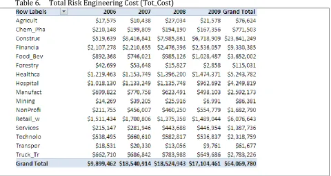
Table 6. Total Risk Engineering Cost (Tot_Cost) ... 11

Table 7. Correlations for Scatter Plot Matrix ... 14

Table 8. SIC Category Statistics ... 22

Table 9. SAS Output: Identifying Covariance Structure ... 29

Table 10. Covariance Structure Output ... 30

Table 11. Primary Model Output: Initial Solution ... 32

Table 12. Primary Model Output: Final Solution ... 33

List of Figures

Figure 1. Basic Work Flows for Risk Engineering Activity ...2

Figure 2. SIC Organization ...4

Figure 3. Scatter Plot for Continuous/Ranked Variables ... 13

Figure 4. Scatter Matrix of Transformed Variables and Service Year with SAS Code... 16

Figure 5. Histogram Comparisons of Dependent Variable ... 17

Figure 6. Log Transform and Box Cox Transform ... 18

Figure 7. Profile Plots for SIC Levels and SAS Code: Ln_loss by Year ... 20

Figure 8. SIC Category Level Profile Charts and SAS Code... 21

Figure 9. Illustration: Between , Within Effects ... 24

Figure 10. Iterative Process of Data Fitting ... 25

Figure 11. Residual Diagnostics: Correlated Residuals ... 33

Figure 12. Corrected Residuals: Accounting for Correlation ... 34

Figure 13. Industry Group Profile Charts: Predicted by Model ... 34

Figure 14. Industry Group Profile Charts: Sample Data ... 35

Figure 15. Cook’s D ... 36

1. Introduction

1.1 Background Information and Context

The primary author of this research has a 24 year career history, in commercial insurance risk

engineering, and the following comments, providing background information, result partly from

that experience .

In the casualty/property insurance Industry, the role of risk engineering is widely recognized

as critical in delivery of financial services by insurance underwriters. Typically this role

encompasses these tasks in the insurance production sequence, underwriters follow to provide

insurance policies:

 Surveying prospective businesses to assess future claims risk.

 Consulting with insured companies to reduce losses.

 Investigating claims to learn preventive measures (not to financially settle claims).

 Completing data analysis to determine long-term trends.

There are many specialists in risk engineering, such as boiler inspectors, fire inspectors,

ergonomists, industrial hygienists, transportation specialists. (National Safety Council, 1992). For

the reader interested in the roles played by risk engineering in the insurance industry, one might

begin with one of a number of professional organizations, such as ASSE, at www.asse.org, or a

second industry organization, the Board of Certified Safety Professionals, at www.bcsp.org.

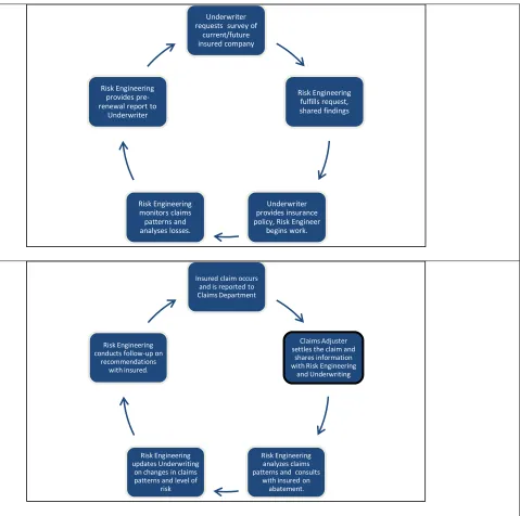
The flow chart below illustrates two basic production processes in casualty/property work

cycles, and some of the most important roles filled by risk engineers. First of these is the insurance

policy cycle, in which risk engineering has a survey role. Second is the claims cycle, in which the

risk engineer acts as consultant to intervene and prevent loss (Head,9). This research investigates

Figure 1. Basic Work Flows for Risk Engineering Activity

It is an ongoing discussion in the industry to develop credible methods, to measure benefit of

risk engineering expense, in terms of reduced claims cost or frequency. Risk engineers fulfill

various critical roles in the casualty/property insurance industry and the challenge of assessing

financial impact resulting from these is the purpose of this research.

Underwriter requests survey of

current/future insured company Risk Engineering fulfills request, shared findings Underwriter provides insurance policy, Risk Engineer

begins work. Risk Engineering monitors claims patterns and analyses losses. Risk Engineering provides pre-renewal report to

Underwriter

Insured claim occurs and is reported to Claims Department

Claims Adjuster settles the claim and

shares information with Risk Engineering

and Underwriting

Risk Engineering analyzes claims patterns and consults

with insured on abatement. Risk Engineering

updates Underwriting on changes in claims patterns and level of

risk Risk Engineering conducts follow-up on

1.2 Purpose of Study

While there are general strategies of measurement, there is no single, easily-applied,

widely-accepted, measure to calculate financial benefit from risk engineering activity (National Safety

Council , 1992). One possible means of creating such a metric is a statistical model, powerful

enough to associate a wide variety of risk engineering data, with claims data of the customers

serviced by risk engineering. Such a model, using a wide-scope sample over many types of

companies, might provide the statistical insight, to draw conclusions on how risk engineering

impacts customers, financially.

Since risk engineering service might occur over months or years for a given company, financial

impact resulting from this expenditure may become evident gradually, only after years.

Accordingly, it makes sense to utilize a data model which measures the association over time,

between risk engineering activity and claims occurrence. A longitudinal model seems appropriate.

1.3 General Description of the Data Sample

Inputs in the model, the independent variables, are of four types.

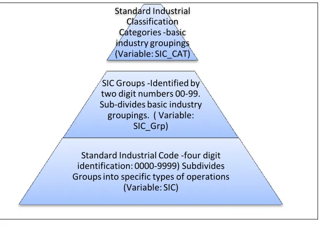
 Basic Information on the insured company, including the type of business enterprise, and location (state). The variables in this group are of several levels of Standard Industrial

Classifications, and give a basic identification of the type of business enterprise. This will

prove important throughout this research.

Note, obviously, for reasons of data security, all names of insured companies and other

identifiable information have been removed. Origin of these industry groupings is the U.S.

Government Bureau Of Labor Statistics, as noted in the following link: www.bls.gov/pub,

Figure 2. SIC Organization

It should be noted this classification system has been updated to the newer NAICS version

on the National Bureau of Labor Statistics website; however, the SIC classification system is

still used in the insurance industry, as is the case with the insurance company providing

the data.

 Basic underwriting information, including names of insured companies for every year of data, and the premium paid per year.

 Financial information pertinent to risk engineering activity, including budget expended per customer and the basic types of activity: that provided before the insurance contract, or

during it. We also knew the time (in months) each customer was provided service. It is

common for underwriters to survey future clients, and have detailed on- site risk

engineering surveys completed. Outcomes and findings of these prospective surveys assist

to decide if coverage is to be provided and under what conditions. Prospected companies

may be required to make changes in operations, to minimize risk in order to acquire

coverage: these changes may affect future claims patterns for the better.

Standard Industrial Classification Categories -basic industry groupings (Variable: SIC_CAT)

SIC Groups -Identified by two digit numbers 00-99. Sub-divides basic industry groupings. ( Variable:

SIC_Grp)

Standard Industrial Code -four digit identification: 0000-9999) Subdivides Groups into specific types of operations

 The choice for output variable (the response variable) is total dollar claims costs paid to settle claims per year for the insured company. There are many choices to use as the

response variable (count of claims, ratio of count of claims to dollar loss, etc), this choice is

intuitive and simple. Dollar loss per customer per year is valued as of 12/31/2009. For

those not familiar with casualty/property insurance claims, valuation of claims data is an

important detail, since claims dollars frequently change in value over a period of years.

Insurance insiders refer to this as “claims development” (Head, Essentials of Risk Financing,

1996).

1.4 Challenges

As a veteran of the industry, this author is unaware of any serious attempts to build such a

model. Understandably, there are a number of natural obstacles to prevent this, such as:

1. Typically, data fitting is an easier task if the observations, or data points, are independent.

In other words, they are unrelated statistically. While this would be plausible for two

distinct companies for one year, most of the companies in the sample data had multi-year

associations with the underwriters. Hence, repeated years of claims experience must be

considered related and dependent. This type of data is considered clustered or repeated (or

longitudinal), and requires some special techniques to account for data dependency (Diggle

et al, p 17). The statistical relationship, expressed over years, is time-dependent and may

change substantially, over time.

Because the data is time-dependent, complexities in analysis are introduced. Of prime

concern is the type of correlation (positive or negative) between the claims costs and the

independent variables, including risk engineering expense. With time-dependency, at some

times this correlation may be positive, and other times negative. A chief interest in this

2. A second challenge to building such a model, is the presence of other more powerful forces

at work, which could mask or hide financial impact of risk engineering involvement.

Statistically, this involves the issue of scale: and differences of scale are manifested in

various forms. One of these results from the fact that some business activities are much

more hazardous, inherently, than others and are likely to generate more serious claims.

For example, working at heights in construction, obviously is much more likely to produce

serious falls than typical office work. (Professional Safety . February 2004 p 25, Injury

Ratios). These differences in claims costs may be orders of magnitude. While much effort is

expended to make hazardous work safer, these different levels of risks and resulting claims

trends are more or less permanent , and pervasive.

3. A third challenge of this project also pertains to differences of scale of financial influence.

Typically, risk engineering budgets are very small compared to overall claims costs and

insurance premiums, as depicted in the tables 3 and 4. Logically, one would expect less

influence on the financial dynamics, resulting from risk engineering budgets, compared to

larger economic forces present. As a result, the statistical relationships involving risk

engineering expenditures may be hidden, unless the statistical model is sufficiently

sensitive to filter through these larger forces, and reveal correlations between risk

engineering and claims costs, over time.

4. A fourth challenge of data-fitting and the subsequent model, results from the potentially

transitory nature of insured-underwriter relationship. Typically, in the U.S., insurance

contracts have 12 months duration, and companies are free to find the best contract in

insurance coverage, periodically. This can result in discontinuity of risk engineering service

from a single source, since the risk engineering service characteristically changes with the

insuring company. From a statistics perspective, this creates the issue of missing

impact measurement. Those conducting statistical research must choose appropriate

methods that work, with data with some missing observations. Table 1 below shows the

sample data: uneven counts across the four years indicate drops in coverage, new clients

etc.

There are statistical methods to deal with this type of data. Importantly, the Mixed

Procedure of SAS 9.2 fits longitudinal data with observations missing at random, as is the case

with the data used in this research. Procedure Mixed in SAS 9.2 fits data to the Linear Mixed

Model.

1.5 Development Path of the Report

Development path of the report includes the sequence:

1. Description of the raw data and the variables chosen to be in the model.

2. Preparation of the data for use, by making necessary transformations to the variables.

3. Creation of the model, running the model and examining the output.

4. Evaluation of the fit of the model.

5. Interpretation of the results applied to the initial questions.

2. Raw Data and Variables

2.1 Basic Characteristics of the Data

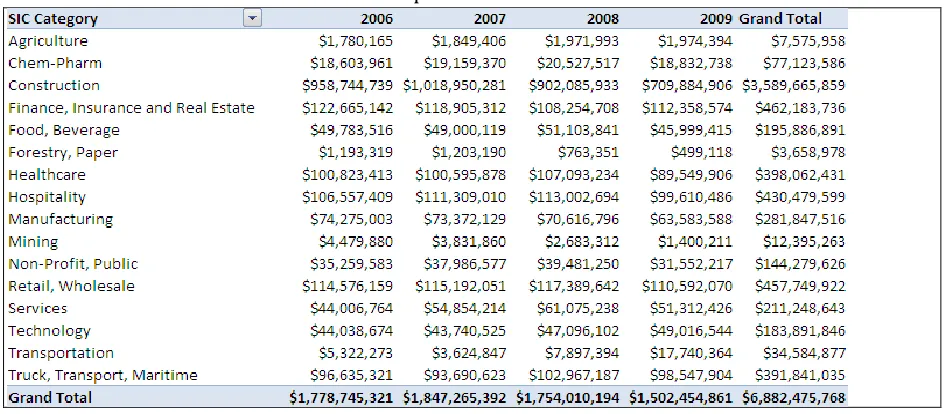
Table 2 below shows overall dollar sums of the raw sample data. A large amount of customer

data was made available in 2010 to conduct this research. At our disposal were 138,955

records of data, each representing one year of the four year period for most types of customers

provided insurance contracts. Consistent grouping of data was by industry groups, in Tables 1

through 6. Initial filtering of the data was required to insure data consistency, as noted:

 All observations with negative earned premium or negative risk engineering cost. These amounts are negligible and reflect some accounting practices which can result from

revisions, from audits.

 All observations for year 2010: these are projections of 2009 data (premium, etc).

 We filtered the data to only use companies from SIC’s in which there was a minimum level of activity over the course of the four years. Thus, we excluded all SIC’s in which there were

less than five observations (five customer-years). Additionally, we chose only observations

for Standard Industrial Classifications which, stayed fairly constant through the four years.

The approach here was to minimize or control dramatic increases or decreases of customer

counts, resulting from the introduction of new types of industries, or dropping or

phasing-out coverage with certain industries. It is not uncommon for Insurers to withdraw from

specific markets or industry types for business-strategic reasons.

The above steps left 14,766 observations. Using this, a random sample was selected for 50% of

these rows to be used in the thesis: 7347 observations.. Validation of the model was completed with

the remaining 7422 observations.. We collected the initial random sample in the source file, an

Excel 2007 file. After this step, all further analysis was conducted in SAS 9.2

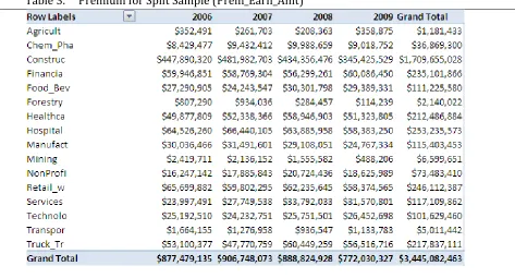
Premium Earned (Prem_Earn_Amt) appears below, grouped by calendar year and SIC Category.

Table 2 is for the entire sample and Table 3 shows that for the split sample. Table 5 and Table 6

show various Risk Engineering Costs. The data differentiates types of Risk Engineering Costs, with

Table 5 showing costs for surveys conducted at the request by underwriting, before insurance

coverage was contracted. Table 6 shows all costs during coverage time, the ratio of these two are

Table 1. Overview of Sample Data: Entire Sample by Year and SIC Category

Table 3. Premium for Split Sample (Prem_Earn_Amt)

Table 5. Risk Engineering Cost: Prospect (Prospect): Pre-Coverage Surveys.

2.2 Data Variables

Throughout this research paper, all variables (fields) of data will be of three basic types:

(1)Class Variables, such as SIC, Industry Classification, location (State) or subject (customer).

Here, the term “level” refers to subgroups of class variables.

(2)Continuous numeric variables, such as premium, claims dollar loss, etc. Many of these are

currency, those which are not will be apparent in the usage.

(3)The time variables used are calendar year and service year.

Detailed definitions of all variables used in the research are to be found in Appendix A.

2.3 Relationships of Variables

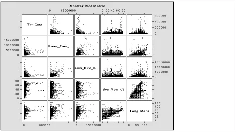
Visual exploration of continuous and ranked variables appears below. Visual data analysis we

accomplished, primarily by use of histograms, QQ-plots, and profile charts. For Figure 3, each of the

smaller panels are scatter plots comparing two variables, horizontally and vertically. Legend for the

names shown on the diagonal are:

Tot_cost---Dollar cost for risk engineering activity. Each dot represents a customer year.

Prem_earn---Earned premium in U.S. dollars for every customer for every year.

Loss_best_est_amt---Claims dollars for each customer/year.

SVC_mon_ct---Service month Count for customers.

Long_mons---Total time of insured time (in months) for the given customer.

Essentially, we wished to identify patterns or basic shapes in the scatter. Patterns occur for:

1. Tot_cost and Prem_earn. This type of wedge shape suggests a data relationship which may be

useful.

2. Prem_earn and Loss_best_est_amt (yearly claim dollar loss). Note the pattern here is distinct

3. Tot_cost and Loss_best_est_amt. One should note the rough scatter shape is approximately the

same as the first.

With the scatter plot in Figure 3, our greatest interest is any patterns associating the dependent

variable (Loss_best_est_amt) and the potential regressor variables, also occurring in the Figure.

We see there are some rough patterns and shapes apparent, along the first column of the Figure,

and these suggest an underlying statistical relationship is present.

Figure 3. Scatter Plot for Continuous/Ranked Variables

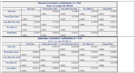
In Table 7, our interest is observation of any relationships between the claims cost, our

response variable, and any of the others. While the Pearson correlations are strong between the

time variables, as a group, the time variables do not correlate highly with claims cost.

The highest correlation coefficient exists between premium and claims cost. This is to be

expected: considerable expertise among actuaries and underwriters result in a strong relationship

between Claims Cost and Premium. Actuaries build statistical models to forecast claims loss, and

higher results indicate that the two variables are ordered similarly (For two variables x and y,

higher x variable means higher y variable). No time variables rank relatively high with claims cost.

The high amount of correlation of premium and loss, apparent in the table, will assure that a

high level of regression will emerge in a basic linear model, assuring some success in creating this.

However, this strong relationship can also hide the relationships of greater interest to us:

relationships directly controlled by risk engineering.

It is appropriate at this point to note that modeling premium and claims costs are not subjects

of this research, and we accept these variables as necessary components of the statistical setting of

risk engineering. It would be possible to build a model without the premium variable, but premium

is very much in the context of risk engineering work, and to ignore it is not logical. In some cases

underwriting decides risk engineering budgets as a percentage of the annual premium .

We anticipate the effect or impact of risk engineering may be much less than other effects, given

previous discussions of scale, but assessing this is a chief interest. We also desire to incorporate all

possible variables of interest into our model, to increase its explanatory capability.

The scatter patterns of financial variables in Figure 3 suggest a simple transformation (natural

logarithm). We apply this to the variables and the resulting scatter pattern is shown below in

Figure 4. We note that logarithm transform assists with the scaling issue mentioned. Finally, the

scatter matrix previously showed many points which appear to be outlier points, and the log

transform will help control outliers. Additionally, we introduce a fourth financial variable, the log

value of the prospect report cost. We applied the transformation f(x) = ln (x +1) with the variables:

Ln_loss = ln(Loss_best_est_amt +1)

Ln_Cost= ln(Tot_cost +1)

Ln_Prem=ln(Earn_prem)

Ln_Prospect = ln(prospect +1).

Note, addition of one unit to each variable was necessary to make sure the logarithm was

defined for all observations. These transformations show a diffuse linear relationship among many

of the matchings of the variables of interest. We are chiefly interested in associations between the

dependent variable, Ln_loss, and the independent variables. Also, one of the time variables (Svc_yr

for service years) has been included (0-7) and some relationships are present here.

In Figure 4, while the log-transformed risk engineering finanical (ln_cost) has an approximately

normal distribution for most of the observations, there are many customers which have $0 risk

engineering expenditure. This variable may be multi-modal (more than one center) in distribution.

While the pattern is diffuse, the roughly diagonal direction of the scatter matrices indicate a linear

Figure 4. Scatter Matrix of Transformed Variables and Service Year with SAS Code

2.4 Exploration of Distribution of Variables

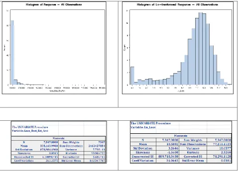
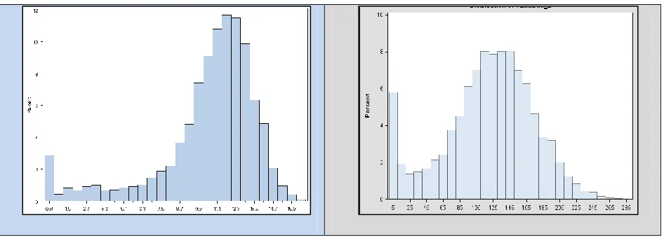
An examination of Histograms for the claims lost below, shows widely scattered distribution of

the points and suggests that the financial variables may have exponential distributions. The scale of

the axis shows the great extent of outlier points. Introducing a logarithm transform f(x) = log (x +1)

greatly reduces the spread of the data, compared to the mean. Comparing mean and standard

deviation of the raw data and the transformed data in Figure 5 shows the effectiveness of the log

transform to cluster the data and reduce the spread of the data. (SAS 9.2 User Guide, Univariate

Inspection of the graphs also suggest a multi-modal distribution, with most of the data

clustered in a roughly normal distribution around a center of 12. There may be a second cluster

center of data, which accounts for the lower valued claims.

Figure 5. Histogram Comparisons of Dependent Variable

At this point of data exploration, we conclude that the linear mixed model is a plausible model

for this research. We conclude this, since histograms indicate linear relationships are present in the

data and the data is longitudinal in type. The linear mixed model is an appropriate choice of model

for data having these attributes (SAS 9.2 User Guide, 2008).

Later in this research we will explicitly define the specifics of the linear mixed modal and verify

3 Exploratory Phase: Data Transformations

3.1 Box Cox Transform

Up to this point of the research, the only data transformations applied are the simple log

transformations, to cluster the data. Other methods of transformation of the data can enhanced our

ability to fit the data. One of these is the Box-Cox Transform (Montgomery P 171). Earlier we noted

the approximate normal distribution of the ln_loss variable (the transformed claim cost). This can

be enhanced For a given variable y, this is defined as:

f y y f f y y f

The SAS 9.2 Procedure “Transreg” finds the optimum choice of λ= 2 by minimizing the residual

sum of squares between the response variable and candidate power curves. Applying this

transformation to the response variable ln_loss (the claims cost) . and running the Univariate

Procedure to generate the Q-Q plots and the histogram for all of the sample data, we generate the

following results, shown in Figure 6, compared to the previous distribution. The new result better

approximates normal distribution, based on visual inspection, and is more symmetric. Note we

have introduced tln_loss_trans: the new Box-Cox transformed response variable.

3.2 Data Exploratory Phase- Profile Analysis

The final phase of data-exploration is a detailed examination of profile graphs: these are line

graphs, with the horizontal axis being the years, and the vertical axis being the claims costs.

Examination of these graphs is essential for longitudinal data sets, since this type of graph is suited

to show movement of the data over time. (Diggle, p 33) However, the chief challenge of using this

type of visualization with a large data set (7337 observations from 2235 customers) is the clutter

and statistical noise, which obscure important patterns of data. Understanding of the patterns of

movement of the data across the four years will be essential to correctly specifying the model.

One obvious solution to the problem is clustering the observations using the Standard

Industrial Classification coding mentioned earlier. The following two graphs in Figure 7 show

profile plots for two levels of this classification. Note the graph in Figure 7 is longitudinal in scale.

There are 73 four-digit SIC Codes represented in the data in the first panel. We note the

between-class variance (the spread of the lines) appears to reduce as the years increase. Non-constant

variance cannot be handled by basic linear regression methods, but linear mixed models can deal

with this data feature. Figure 7 shows the profile data at the SIC level and a higher level in the

second panel, at the SIC_Cat level.

The change of variance over the four years becomes clear when we examine the data at the

SIC_Cat level (the general industry level). The non-constant variance noted across the years is

partially a reflection of dollar claims development. Generally, a serious claim with large dollar

amounts, will mature and change in value, over some years, before it is settled and closed.

Additional complexity is introduced in the issue of claims development when IBNR ,“Incurred but

not Reported”, is considered. Serious claims and claims under litigation further complicate

forecasting. The reader can contrast the two profile charts in Figure 7 to see some of this effect.

The financials in this study are “Point in Time” financials. All claims data is dated 12/31/2009.

Therefore, serious claims occurring three years before, have had much more time to mature

financially. This effect is one of the justifications to utilize a longitudinal model, which clearly

illustrates the difference in variance between years. Additional evidence of change of correlation

and covariance will be discussed with the variance/covariance lag analysis, to follow in Part 4.

Figure 7. Profile Plots for SIC Levels and SAS Code: Ln_loss by Year

Cumulative effect of data transformations used in this research, on the profile charts, appear

below in Figure 8. Shown are: the original data profile, log- transformed, Box-Cox transformed, as

well as standardized. With all of them, we see inconstant variance over the years, mentioned

before. The transformations appear to reduce difference of variance in data across the years: a

desirable effect. Additionally, they appear to be roughly parallel. This question of profile data

pattern will be revisited in the following section on covariance structure. Note that panels 2, 3, 4

(left to right) in Figure 8 do not show 95 observations from the Agricultural SIC_Cat. This was

sacrificed to provide additional resolution of the data for most of the SIC_Cats. Note also, the entire

Figure 8. SIC Category Level Profile Charts and SAS Code

From Figure 8 we note that the Box-Cox Transform reduces the change of variance over the

years, which assists in fitting the data. Nevertheless, the Figures may suggest that the data is more

orderly than it is, in reality. The SIC Categories do not differentiate the data as cleanly as the

profile charts would suggest.. The output of the GLM Proc generated by the code (without

SIC_Cat level for each year. Categories with Standard Deviation more than ½ of the Mean, have

questionable value in grouping the data.

Table 8. SIC Category Statistics

Level of N Loss_Trans

SIC_Cat Mean Std Dev

Agricult 94 14.8608 22.3671

Chem_Pha 85 63.5952 35.7667

Construc 3274 79.5982 22.9789 Financia 618 57.9816 30.3298 Food_Bev 183 67.0968 35.8816 Forestry 15 66.3212 16.4651 Healthca 422 62.7314 32.9126 Hospital 721 69.0493 24.3168 Manufact 347 66.2396 30.0852

Mining 12 80.4465 20.3243

NonProfi 259 59.7081 31.3577 Retail_w 669 65.6005 29.5933 Services 164 73.8625 30.3737 Technolo 205 75.4836 27.9877

Transpor 10 77.1334 31.4603

Truck_Tr 266 72.2398 37.4372

4 Model Construction

4.1 Basic Concepts for Linear Mixed Model

The following section provides a non-technical introduction of data models , applicable to the

general linear mixed model. In that context, these comments serve to provide a high-level look at

the unifying concepts for statistical modeling, at least in terms of the linear mixed model. Some

basic examples appropriate to the flow of this research will be used. We will follow with the

technical formulations for the model in section 4.3.

Recall the goal of this research paper is to fit the sample data presented earlier, to a data model.

than a structure of steel and concrete, our end-product will consist of equations, tables and other

mathematical objects. While the end-purpose of the engineer, of building a high-rise building, is to

provide a suitable interior space for business offices, the end-product of the Statistician in building

a data model, is to identify the patterns and structure of the data, to describe these. The end

purpose of the statistical model is forecasting or prediction.

There are many statistical models than can be used in data fitting for this, but the linear mixed

model is a powerful type of model, since it accommodates different types of quantitative

relationships between variables or effects. The key term used here is “effect”: the concern is with

the type of effect and the strength or magnitude of the effect. Four types of effects are prominent in

the mixed model: “Within Effects”, “Between Effects”, “Fixed Effects”, “Random Effects”.

To illustrate these in the context of this paper, consider the operations of three companies over

three consecutive years: company A is a construction operation, company B is a manufacturing

operation, and the company C may be a transport company, as shown in Figure 9. The statistical

models at our disposal can identify and quantify all of these effects. The diagrams in Figure 9

illustrate at least 15 different effects, counted separately, and we are ignoring factorial (cross)

effects. Typically, averaging of these effects by type or group is normally completed.

In addition to “between” and “within” effects, Statistical tools in SAS can identify and measure

fixed effects and random effects. (Diggle, 2002). Fixed effects can be characterized as definite and

precise. The simple linear relationship of Y = 2X + 5 models a fixed effect between the two

The longitudinal correlation for claims rate of the same customer is depicted as the “within effect”. Overall, this effect would be independent of correlation or relationships with similar companies. We would expect a greater overall effect with this, compared to dissimilar operations (other Industry Groups).

Arrow Up : “between effect”. We would expect some correlation of claims rates, even though the operations are different: the year is the same.

Commonalities pertinent to general economic conditions, or geographic location might be considered “between-class effect”. In our data, two chief

between-class effects are service year and year. Initial analysis of the geographic relationship did not indicate importance of the location “State”, variable.

Arrow up: here is a second “between effect”, which differs from the earlier, given a different year. As a fixed effect, this would be combined for all years.

Said otherwise, we are dealing with different types of data dependency, and correlation. Magnitude may vary greatly, but the overall success of the model is largely a result of our degree in identifying and measuring these different effects.

Figure 9. Illustration: Between , Within Effects

On the other hand, random effects intrinsically involve the notions of random variables

distributions, mean, and variance, With the scatter plots shown in Figure 4, the characteristic

normal curve shape we see, is a random effect between claims dollar loss (transformed) and the

probability of specific magnitudes of loss. This random variable shows the claims costs which are

more probable, occur in the center of the curve.

• Year 1 • Claims Compan

y A

• Year 2 • Claims Compan

y A

• Year 3 • Claims Compan

y A

• Year 1 • Claims Compan

y B

• Year 2 • Claims Compan

y B

• Year 3 • Claims Compan

y B

• Year 1 • Claims Compan

y C

• Year 2 • Claims Compan

y C

• Year 3 • Claims Compan

4.2 General Data Fitting Method

Several of the above cycles were needed to fit the final version of the data. Some comments for each of the above steps are as:

1. The subject is the Acct_id (customer) and the Repeated effect is the year of coverage 2006 – 2009. Our Fixed effects include the Class variable ( SIC_CAT), ranked variables (Svc_yrc for service year) and continuous variables (Ln_prem-transformed premium, Ln_cost- transformed Risk Engineering Cost, and Ln_prospect, transformed prospect costs). Year is our repeated effect variable and is used as a class variable.

2. We control random effects primarily by choosing a covariance structure, suggested by the profile plots and other data exploration as detailed in section 4.4. The three most promising types of covariance structure were found to be auto-regressive moving average (“ARMA(1,1)”), CS (“Compound Symmetry”), and Ante-Dependence (“Ante(1)). Later we show how we made the final choice.

3. Several SAS test outputs are used with each choice of variance structure for the random effect, including the Null Likelihood, AIC and BIC tests. These are some tools to measure our success.

4. AS we run the SAS code, we also desire the F test results for the fixed effects variables to have low p values, and desire the AIC, BIC and Null Likelihood to reduce, or stay level, as other changes are made. This process we run as many iterations we need, until we cannot improve on the test results noted above.

Figure 10. Iterative Process of Data Fitting

At this point we have identified essential patterns of the data and can begin to fit a model. Two

suppositions are reasonable at this point, but we verify them after building the model:

1:Select Fixed Effect Variables, Subject, and Repeated Effect 2. Select Covariance (Random Effects) 3. Test Covariance for

Fit to Data 4. Test Entire

Model for fit: stop process or

1. We have sufficiently met the requirements of the linear mixed model, that the response

variable is associated linearly with the regressor variables.

2. We have identified important candidates for “Between”, “Within”, “Fixed”, “Random”, and

“Repeated effects” such as year, SIC_Cat, service year, and customer.

In selecting specifics of the model, we follow basically a four stage process (Diggle, 2002)

illustrated in Figure 10.

After arriving at a reasonable model, in terms of SAS output, many diagnostic tests are

available to check for outliers, influential observations and residual analysis (SAS User Guide,

2008). We provide this in a later section.

4.3 Data Model Definition

The linear mixed model builds on the general linear model characterized by the equation:

y = Xβ + e

With y, as a vector of response variables; X, as a matrix composed of the regressor values; e,

the residual value vector containing the error terms; and β, as the vector of coefficients, derived as

a solution. The assumptions are that y has normal distribution, and e also has multivariate normal

distribution with mathematical expectation, E(e) = 0 and variance, var(e) = σ2_I.

The linear mixed model relaxes some of the requirements of the general linear model.

(Henderson, 1984). This is done by introduction of an additional vector of multivariate normal

random variables, u, into the equation above. As is the case with the regressor matrix X, Z is

assumed to be a known set of variables which are given. “e” retains the same meaning as before.

The resulting expression is:

y = Xβ + Zu +e

With the new quantities we also make these assumptions:

u

_{e =}

V = Var(y) = ZGZ’ +R

The ultimate goal is to determine estimates of β and u specified in equation (2). However, this

problem is made complex and difficult, due to the fact that we may not know the actual G and R

matrices, and these must be estimated. This problem is not within the scope of this research, and

the reader can see relevant research (Henderson, 1984). Note however, that the general strategy

for solution is to solve the general least squares problem:

[y-(Xβ + Zu)]’( V-1)[y- (Xβ + Zu)] (6)

The mixed model equations result, and these are:

_u =

_y (7)

We use the method of Restricted Maximum Likelihood to minimize error in (6) and derive the

estimates for R: and for G: as shown in (7).

The solutions of the mixed model equations are:

_{y (8)}

u Z’ _{(y-X (9)}

The version of the Mixed Model used in this research is a simplification of the standard model

provided above in (7), (8), and (9). (Jennrich and Schluchter, 1986). We write this model as :

Y

~MVN(X

,V

).

Effectively, equation (10) expresses the claims costs , Yi , for customer i, as a multivariate

normal, random vector with expected value

X

and variance/covariance matrix V

.

multiple regression linear model with correlated errors within each subject (Customer). Effectively,

we are allowing the possibility that the claims costs for a given customer are correlated across the

(2). However, our experimentation showed no advantage for this additional complexity, in terms of

fit. Rather than modeling between-class effects (such as that between SIC Categories) using the u

d m vect , these effects e m de ed by the fixed c mp e t.

We add subscripts to provide additional information and express this simplified model

alternatively as:

,

=

+

Note, n = total observations, and k = number of regressor variables. Since we are using

longitudinal data, it is helpful to think of the data as a set of repeated measures (years) with

customers: for i = 1,2,3. . . m customers. The X symbol is the matrix composed of the regressors

(Ln_Prem, Ln_Cost, etc). β is the vector of coefficients for the fixed effects. The r vector in (11) is a

multivariate normal vector with expected value of 0 for each customer- year of data and is the error

term.

Therefore, the V matrix above can be considered as a block diagonal matrix, with each block

associated with a customer. For each customer in equation (8), the equation above becomes:

,

=

+

The number of observations in each of the m blocks can be 1, 2, 3,or 4, depending on the

number of years in the history of the given customer. The Covariance/Variance matrix of the

residual vector r, for each i, i = 1. . . m, is _,

,

this simplification, we also have:

E = 0, a zero- valued vector. (13)

4.4 Covariance Structure

After the exploratory analysis of the earlier sections, it is necessary to specify the

variance/covariance structure, the

V

= V

(14)

This will be a block symmetric matrix, each Vi block will correspond to individual customers as

specified in equation (12). Essentially we need to choose a structure that will capture the pattern of

the data across the years. In addition to the previous exploratory analysis, variograms or

covariance/correlation lag analysis between the years can be helpful in determining the

distribution of variance across the years of the study (Diggle, 2002). There may be more than one

adequate choice of variance structure, but a serious error with model specification will produce

unsatisfactory end results.

Table 9. SAS Output: Identifying Covariance Structure

With this in mind, we run PROC Mixed, specifying no variance structure for the solution and

output the covariances between the years. This will output the covariances between the years and

variances of the years as shown in Table 9.

The SAS output (using the R and Rcorr options with the Repeated statement) provides the first

individually. The second block of the same table arranges these covariances in the specified order,

by the pairs of coordinates. Then, we calculate correlation:

ρi,j = Cov(ri,rj)/(σiσj), (15)

These results are shown as the final blocks of numbers, of Table 9. Thus, as an example, the

correlation between year 2007 and year 2009 is .3165, as shown in the last block of numbers. From

this information, we conclude that the covariance and the correlation have a roughly linear

relationship, and that covariance and correlation are stronger when the years are adjacent in time.

This would suggest several types of covariance structure as plausible, particularly, those based on

various types of moving averages.

After some experimentation, using the method described for fitting in the text with Figure 10,

we derive the Ante(1) model, which is First Order Antedependence, (Kenward, 1987) and (Patel,

1991). Other candidate covariance structures including Compound Symmetry, Variance

Components, Auto Regressive, and others were tried; Ante(1) had best results in terms of fit.

Table 10. Covariance Structure Output

The SAS 9.2 output for the covariance structure appears in Table 10. These are used to compute

the Vi blocks for the V matrix. Note our ” V” is the same as the “R” in SAS output. First block in the

table 10 shows the R Matrix values, the Vi . In the SAS Code we requested the Vi block for Customer

block will be identical. Ante(1) collapses to produce a smaller block for customers with less years

as discussed immediately.

It is important to note the definition of Ante(1): , (16)

<1, the kth _{autocorrelation parameter and}

is the ith variance parameter.

th ee dime i s this w u d be e ized s

.

4.5. Model Specification

Table 11 shows the original solution output of the SAS code provided in the Appendix. We note the

Null Likelihood Ratio Test is acceptable, however, some of the levels of the SIC_Cat, (the Industry

groups) do not meet needed level of significance, to remain in the model. Therefore, the model we

run again, grouping all those groups into a miscellaneous category. The result is approximately the

same AIC, AICC, BIC and Null Likelihood test and the all remaining groups meet the .05 level of

significance. Ln_Cost is improved in p value, but might be considered marginal in the second

version. Results of this second run can be found in Table 12.

Figure 11 and Figure 12 following, show diagnostics of the fit. An important assumption of the

linear mixed model is that the residuals are multivariate normal in distribution, the diagnostics

below basically confirm this assumption, although there is some deviation from the assumed

distribution. The first panel in Figure 11 shows graphs of the raw residuals. However, these do not

take into account that the residuals are in fact correlated, and we should not expect the normal

patterns on the graphs: completely normal distributions should produce a random band of points

grouped around the 0 horizontal line (Gregoire, 1995).

Residual Diagnostics generally are more complex with the Mixed Model, compared to the Linear

Var(Y) = V (17)

Var(Y) = ’ (18)

= ’-1 _{* r (19)}

V is our block diagonal covariance matrix introduced earlier. Since V is Positive Definite and

Symmetric, it can be factored as a Cholesky Decomposition (first factor is lower triangular, second

factor is upper triangular, lower triangular has positive diagonal elements) : r c is the result. It is

uncorrelated. Figure 12 shows the scatter plot with this formula applied and the pattern of scatter

more closely matches a random appearance.

Table 11. Primary Model Output: Initial Solution

Figure 13 and Figure 14 compare the profile graphs of the predicted data and the actual data.

While the predictions mimic the general pattern of the raw data, some disparity is evident. We

noted earlier that the SIC_Cat field has limitations as a predictor. The amount of disparity is

Table 12. Primary Model Output: Final Solution

Figure 12. Corrected Residuals: Accounting for Correlation

Figure 14. Industry Group Profile Charts: Sample Data

4.6 Influence Diagnostics

As is the case with previous residual diagnostics, influence diagnostics is more complex than

that with the standard linear model. (Gregoire, 1995). Estimates of the fixed effects and the random

effects are linked, removing points for influence diagnostics, require refitting all of the data left to

achieve a completely new solution, both fixed and random. SAS provides the option of estimating

revised β parameters without refitting the entire model, by asking for no iterations in the

calculations. This is not preferred to the iteration process, but is offered as an alternative when it is

not possible to do otherwise. There is no attempt to redefine the random effects. Cook’s D is

defined in the mixed model as

The reader will note this is similar to the definition of Cook’s D, for the linear model

(Montgomery, 2006) . The “u” subscript indicates the new beta parameters, without the deleted

points in the model. Cook’s D should be interpreted as an F statistic, and if we use the rejection

region of .05, this results in Figure 15 below. We would conclude no points are unduly influential in

changing the β vector, the coefficients. Given n= 7343 observations and with five regressors, the

Cook’s D value required would be greater than 2.10 (F.05,6,120) and this is not the case.

Figure 15. Cook’s D

5: Conclusions

5.1 General Observations

If we compare the output in Table 12, with the original expectations for the model, the general

expectations are met. All of the variables of most interest including the risk engineering cost and

the industry group differentiator, proved useful in the model. Additionally, there were no surprises

in terms of the relative magnitude of them, with premium being by far the strongest effect.

There was no speculation on some available time variables, as noted in the first section, and the

strength of the relationship between service year and claim costs is somewhat surprising: more

service time is associated with higher amounts of claim costs. The impact resulting from prospect

and 2 account for 4986 out of 7344 customer-years, or 68% of the total customer-years

(observations). As such, the graph in Figure 16 helps to understand why prospect service has the

financial impact it has.

Figure 16. Interpretation of Results

5.2 Interpretation of Model

While the Fixed Effects Solutions in Table 12 indicate financial impact in reducing claims cost

over time, for prospect activity, it is appropriate to apply the model to a real-world situation, to

better understand this financial impact. It is incorrect to apply the coefficients in column three of

the solution, as they are, due to the data transformations applied before fitting the data. Recall that

Ignoring random effects, we can calculate approximate results of the model with simulated

data, to better understand the action of the model. To do this, we need to reverse the

transformations applied to the original variables, and insert the solution coefficients from Table 12

in the model. Recall that λ = 2 in the Box Cox Transform. The reader will note that the

transformations (as well as the interpretation of the model) are made more complicated by the

addition of the constant 1, initially when the log transform was used, as well as when the Box-Cox

Transform was applied. The equations below take this into account.

Equation (21) below is the general model with the fixed effects and (22) is the equation with

our values applied. Equation (23) regroups the terms for ease in calculation.

= X

((Ln(Loss_Best_Est_Amt +1)+1)2 -1)/2 = -79.89 + (Ln(Tot_Cost +1) * .103) +

(Ln(Prem_Earn_Amt+1) *12.465) – (ln(Prospect +1)*.1485) + (Svc_Yr * .8194) + (Sic_Cat1 * IN)

(22)

Loss_Best_Est_Amt = (exp(2*( -79.89 + (Ln(Tot_Cost +1) * .103) +

(Ln(Prem_Earn_Amt+1) *12.465) – (ln(Prospect +1)*.1485) + (Svc_Yr * .8194) + (Sic_Cat1*IN)) +1) ^ .5) -1) -1

(23)

Note, in equations (22) and (23), the variable ” IN” = 1, whenever the specific SIC Category is

one of the differentiated SIC Categories {Agricult, Chem_Pha, Construc, Financia, Healthca, Food_Bev

}. Otherwise, IN = 0 as indicated in the output Table 12. This is an indicator variable.

As a real-life example, the following chart uses the above equations to forecast financial impact.

In our situation, we are assuming that the customer is in the miscellaneous SIC_Cat group.

Additionally, we are assuming no risk engineering budget and no service years are recorded. Both

the premium amounts and risk engineering expenditure are plausible amounts. We are therefore

examining the effects of two different amounts of premium and several amounts of prospect

The third column of Table 13 contains output of the equations, immediately above. Of greatest

interest is the last column showing a positive return of investment for some rows. Note we are

using the expected loss as a baseline for calculations. The model predicts maximization of financial

impact in the region of $1000- $7500 expenditure for prospect activity, but this depends on the

premium amount. The fourth column is the ratio of expected loss , at the given level of premium

and prospect, with the first row. Loss percent reduction in column five restates column four as

percent.

Table 13. Simulated Cases of Financial Impact: Prospect Activity

More complex simulations and resulting forecasts, using specific industry groups and non-zero

amount of Risk Engineering budget, could be calculated and would be instructive. This is suitable

Appendix A Data Variables

The following table provides data variable definitions in alphabetical order. The table

distinguishes raw data variables as source variables, from derived variables.

This Readme file provides data definitions for the data files used with the Thesis to build to model. These are ordered alphabetically.

Variable Name Variable Definition

Acct_Addr_St This class variable denotes the US State for the head office for the given customer. Since many customers have multiple locations in multiple states, it was decided not to use this variable in the model. Additionally, insertion of the variable into the preliminary mixed models showed that no states, as levels of this class variable, met a .10 level of significance with t-tests for inclusion.

Acct_has_Prosp_Svc Abbreviation for "Account Has Prospect Service". This class variable (with two levels), shows if any type of Risk Engineering activity occurred for the customer prior to first year of insurance coverage. This is a preliminary survey or survey report, from Risk Engineering, issued to Underwriting to assist in the decision to provide insurance coverage.

Acct_ID Identification number for the customer. After filtering the data as described in the research, there are about 15,000 observations. We split the data into two sub files of the same size and randomly sampled the

observations by Acct_ID.

Assign_Ct This integer valued variable is the total number of assignments completed for an observation (customer-year).

Bus_Unit This class variable is a derived alpha-numeric abbreviation representing the underwriting unit responsible for insurance coverage and was not used in the statistical model.

Ln_Cost: Natural logarithm of Tot_cost, shifted one unit: ln(Tot_Cost +1). The shift by one unit insures logarithm is defined for all observations.

Ln_Loss This continuous variable represents natural logarithm of "Loss_Best_Est_Amt" (shifted one unit).

Ln_Prem This is the natural logarithm of the (Premium Earned Amount + 1). Shift was to insure positive value for this field.

Ln_prospect Natural logarithm of Prospect amount, shifted one unit.

Long_mons This integer variable shows the cumulative amount of time, in months, in which the customer had insurance coverage.

Loss_Best_Est_Amt This continuous variable represents total dollars paid on behalf of a customer for a given year to settle insurance claims. Since claims amounts develop over time due to changes in reserves and other reasons, it is necessary to indicate the point in time the claims were valued: this was 12/31/2009.

in the model.

Pol_Year The integer variable shows the policy year for the given customer. The data sample has observations ranging from 1 to 7 years.

Prem_Earn_Amt Abbreviation for Premium Earned Amount: this is the raw dollar value for all premium on the records for the given customer for a given year of

observation.

Prospect Dollar amount expended in Prospect Service and discussed earlier.

Rec_ID Record identification, observation number for the data. Each row of data represents a customer year based on calendar years 2006 through 2009. The maximum number of observations a customer could have would be four. Sbus_Unit This class variable indicates the underwriting sub-unit responsible for

insurance coverage and was not used in the statistical model.

SIC Abbreviation for Standard Industrial Classification. The variable is a four digit identification and subsets the SIC Groups into 150 subsets.

SIC_Cat Abbreviation for Standard Industrial Classification Category. This is a large scale grouping of the customer into basic industry types. Industry types are abbreviates accordingly: This is a classification variable with 16 levels as indicated in the paper. The nature of the specific industries is indicated in the abbreviated names. SAS truncates names of class variables

SIC_Grp Abbreviation for SIC Group, this subsets the SIC Categories using two digit identifications. There were 48 SIC Groups in the data file.

Svc_Mon_Ct This integer variable shows the cumulative amount of time, in months, in which the customer had Risk Engineering Service of any type.

Svc_Yr: This is a time variable representing the year of service for the given customer for the given observation. The data file has values with range of -3 to 8. A value of "-3" indicates that the observation is for the third year before the customer was placed on service initially. A value of "na" indicates that the customer never had service for any year. Note that the SAS program

transformed this variable and grouped all negative value observations along with "na" as a " 0" value to become the "Svc_yrc" variable. Thus, all "0" value svc_yrc observations correspond to years in which the customer had not Risk Engineering Service.

Svc_Yrc This variable is derived from Svc_Yr and is a simplification. All customer-years in which the customer was not on service were transformed to 0. Loss_Trans Box Cox Transformed version of Ln_loss, the log-transformed claims cost.

Value of lambda = 2.0

Tot_Cost: Continuous positive numeric variable for dollars expended in Risk Engineering activities for a given customer, for a given year for all observations.

Appendix B SAS Code

/*** Reference Figure 4 ***/

/Matching SAS Code for Panel Scatter Plots */

/* Following Code requires changing the infile line to locate data file*/ /* This code creates a group of histogram charts for log-transformed data */

data MD_2011;

infile 'C:\users\Bobby\desktop\DataSample1.csv' delimiter =",";

input Rec_Id $ Acct_Id $ SIC_Cat $ SIC_Grp $ SIC $ Bus_Unit $ Sbus_Unit $ Year Long_Mons Pol_Year Svc_Mon_Ct Svc_Yr $ Prem_Earn_Amt Ln_Prem Loss_Best_Est_Amt Ln_Loss Loss_Ratio Assign_Ct Tot_Cost Ln_Cost Acct_Has_Prosp_Svc $ Acct_Addr_St $ prospect ln_prospect;

run;

/* Create SIC (Standard Industrial Classification Means for Loss_Scaled */

ods html; /*turn on html output*/

ods listing close; /*turn off list (regular) output window, optional*/ ods graphics on; /*turn on ods graphics*/

Data TransMD; Set MD_2011;

/* Renaming service year for consistency */

/* Initial Coding has anticipatory service years */ if svc_yr = 'na' then svc_yrc = 0;

if svc_yr = '-3' then svc_yrc = 0; if svc_yr = '-2' then svc_yrc = 0; if svc_yr = '-1' then svc_yrc = 0; if svc_yr = '1' then svc_yrc = 1; if svc_yr = '2' then svc_yrc = 2; if svc_yr = '3' then svc_yrc = 3; if svc_yr = '4' then svc_yrc = 4; if svc_yr = '5' then svc_yrc = 5; if svc_yr = '6' then svc_yrc = 6; if svc_yr = '7' then svc_yrc = 7; if svc_yr = '8' then svc_yrc = 8; output;

run;

proc sgscatter data=Transmd;

title "Scatter Plots for Loss-Prem-Cost-Prospect Svc_Yrc"; matrix Ln_Loss Ln_Prem Ln_Cost Ln_Prospect Svc_Yrc / diagonal=(histogram kernel);

run;

/* ****************** Code for Graphs Reference Figure 7 ************* */

goptions reset=global gunit=pct border cback=white colors=(black)

ftitle=swissb ftext=swiss htitle=1 htext=2;

/* Input the data: change the infile line as needed */ data MD_2011;

infile 'C:\users\Bobby\desktop\datasample1.csv' delimiter =",";

Acct_Has_Prosp_Svc $ Acct_Addr_St $ prospect ln_prospect; run;

/* Create SIC Category (Standard Industrial Classification Means for Loss Scaled */

proc glm data=MD_2011;

class SIC SIC_Cat Acct_Id Year; model Ln_loss =Year(SIC_Cat); means Year(SIC_Cat);

output out= REmeans2 p=SICmeans; run;

Proc sort data= REmeans2; by Year;

run;

/* Draw plots for SIC Category means by time */

title 'Plot of SIC Category Means Data'; title1 ''Plot of SIC Category Means Data'; symbol1 color=red

Repeat = 76 interpol=join value=dot height=1; legend1 label=none

position=(top left inside) mode=share;

proc sgplot data=REmeans2; xaxis type=discrete;

series x=Year y= SICMeans/ group = SIC_Cat; run;

quit;

/**************Reference Figure 8 ***************************/ /* Bob Parker- Linear Mixed Model for Zurich RE Data 061511 */

/***********************************************************************/ /* Data Input */

ods graphics on;

ods html; /*turn on html output*/ ods listing close;

goptions reset=global gunit=pct border cback=white colors=(red green blue orange) hsize=7.5 IN

ftitle=swissb ftext=swiss htitle=3 htext=2; data MD_2011;

infile 'C:\users\Bobby\desktop\datasample1.csv' delimiter =",";

input Rec_Id $ Acct_Id $ SIC_Cat $ SIC_Grp $ SIC $ Bus_Unit $ Sbus_Unit $ Year Long_Mons Pol_Year Svc_Mon_Ct Svc_Yr $ Prem_Earn_Amt Ln_Prem Loss_Best_Est_Amt Ln_Loss Loss_Ratio Assign_Ct Tot_Cost Ln_Cost Acct_Has_Prosp_Svc $ Acct_Addr_St $ prospect ln_prospect;

run;

/****************************************************/ /* Creating additional variables needed later */

Data TransMD; Set MD_2011;

/* Renaming service year for consistency */ /* Data has Anticipatory Service Years */ if svc_yr = 'na' then svc_yrc = 0; if svc_yr = '-3' then svc_yrc = 0; if svc_yr = '-2' then svc_yrc = 0; if svc_yr = '-1' then svc_yrc = 0; if svc_yr = '1' then svc_yrc = 1; if svc_yr = '2' then svc_yrc = 2; if svc_yr = '3' then svc_yrc = 3; if svc_yr = '4' then svc_yrc = 4; if svc_yr = '5' then svc_yrc = 5; if svc_yr = '6' then svc_yrc = 6; if svc_yr = '7' then svc_yrc = 7; if svc_yr = '8' then svc_yrc = 8; output;

run;

/* ******************************************************************/ /* Running Box Cox to normalize data and standardizing */

proc transreg data = Transmd;

model BoxCox(ln_loss1)= identity(Ln_Cost Ln_Prem ln_prospect SVC_Yrc ); output out = Transmd2;

run; data all;

merge TransMD TransMD2; output;

run;

/* ***************************************************************** */ /* creating SIC Category Mean Groups and Graphing */

proc glm data= all;

class Acct_Id Year SIC_Cat; model ln_loss =Year(SIC_Cat); means Year(SIC_Cat);

output out= SIC_Means p=SICMeans; run;

Proc sort data= SIC_Means; by year;

run;

/* Draw plots for group means by time */