The Interplay of Localization and Interactions in
Quantum Many-Body Systems
Thesis by
Shankar Iyer
In Partial Fulfillment of the Requirements
for the Degree of
Doctor of Philosophy
California Institute of Technology
Pasadena, California
2013
c
2013
Shankar Iyer
Acknowledgements
My five years at Caltech have been among the most wonderful and transformative
of my life. This would not have been possible without the kindness and guidance of
my advisor, Gil Refael. Early on, he gave me the freedom to pursue the problems that
interested me, and throughout my graduate studies, he remained a constant source
of support, encouragement, and enthusiasm. I learned a lot of physics from him, but
I also learned so much more: how to talk to other scientists, how to communicate my
work, even how to organize my notebooks. His personal and scientific influence is all
over this thesis.
Many others enriched my time in the Condensed Matter Group. I particularly
want to recognize David Pekker for being such a patient guide through the intricacies
of dirty bosons. I also want to thank Lesik Motrunich, Michael Cross, and Oskar
Painter for serving on my thesis committee, and Loly Ekmekjian for all her help over
the years. It was very enjoyable to work and learn alongside my fellow graduate
students, among them Paraj Bhattacharjee, Scott Geraedts, Kun Woo Kim, Tony
Lee, Shu-Ping Lee, Hsin-Hua Lai, Debaleena Nandi, and Karthik Seetharam. I cannot
thank Liyan Qiao and Zhaorui Li enough for their friendship and the incredible honor
Liyan, Zhaorui, and Amy transformed our office into a second home and made coming
to work an absolute joy.
Outside of our research group, I am indebted to Hemanth Siriki for putting up with
me for four years. I also want to thank Bill Fefferman, Karmina Caragan, Senthil
Radhakrishnan, and several others for sharing weekend evenings with me. I loved
getting to know Pasadena and the greater Los Angeles area with all of them. Finally,
I deeply appreciate the hospitality that the Nadadur family showed me on so many
occasions during these years. It was great to have such a welcoming home to retreat
to on weekends when I needed an escape from Caltech.
Before beginning graduate school, I spent one year as a Fulbright Fellow at Leiden
University in The Netherlands. I want to thank the Netherland-America Foundation,
Jan Zaanen, and the Instituut-Lorentz for their roles in making that year possible.
I also want to express my gratitude to the Kauffman-Abel family for friendship and
hospitality during that time and during my later visits to Leiden.
From 2003-2007, I was an undergraduate at Princeton University. There, I began
a senior thesis project that eventually expanded and evolved into Chapter 4 of this
thesis. I thank my senior thesis advisor, David Huse, for introducing me to research
in condensed matter theory and for helping me to revive our project when I met
him again at the Boulder Summer School in 2010. I am also very grateful to Vadim
Oganesyan and Arijeet Pal for their insight into the problem of many-body
localiza-tion. During my Princeton years, I made many lifelong friends who still enrich my
Sun, but there are too many others to name.
My interest in physics developed during high school in East Brunswick, and I want
to thank all the excellent teachers who nurtured my curiosity in physics and other
subjects. Moreover, I cannot overestimate the influence of my classmates during this
period. Had I not developed a passion for physics alongside them, I would not now
be completing this thesis.
Before all of this, I had the great fortune of being born into a large, loving family.
Whatever I have achieved would have been impossible without my family’s love and
support, especially in the trying times. Most of all, I want to express my deep
gratitude to my sister (Jayasree Iyer), my parents (Latha and Mohan Iyer), and my
grandparents (A. Chellammal, S. Padmanabha Iyer, N. Jayalakshmi, and H. Sankara
Iyer). However, I also want to thank the rest of my extended family in New Jersey,
India, and elsewhere around the world.
Finally, I want to thank Sowmya and her family for welcoming me into their lives
over the past couple of years. My life has become immeasurably better for having
Abstract
Disorder and interactions both play crucial roles in quantum transport. Decades ago, Mott showed that electron-electron interactions can lead to insulating behavior in materials that conventional band theory predicts to be conducting [105]. Soon thereafter, Anderson demonstrated that disorder can localize a quantum particle through the wave interference phenomenon of Anderson localization [11]. Although interactions and disorder both sepa-rately induce insulating behavior, the interplay of these two ingredients is subtle and often leads to surprising behavior at the periphery of our current understanding. Modern exper-iments probe these phenomena in a variety of contexts (e.g. disordered superconductors, cold atoms, photonic waveguides, etc.); thus, theoretical and numerical advancements are urgently needed. In this thesis, we report progress on understanding two contexts in which the interplay of disorder and interactions is especially important.
Carlo simulations by Hrahsheh and Vojta [70]. We then shift our attention to two dimen-sions and use a numerical implementation of the SDRG to locate the fixed point governing the superfluid-insulator transition there. We identify several universal properties of this transition, which are fully independent of the microscopic features of the disorder.
Contents
Acknowledgements iv
Abstract vii
1 Introduction 1
1.1 Noninteracting Particles in Perfect Media . . . 1
1.2 The Role of Interactions . . . 6
1.3 Aperiodicity and Localization . . . 12
1.4 Disorder, Interactions, and Phase Transitions . . . 21
1.5 Experimental Situation . . . 36
1.6 Overview of Thesis . . . 42
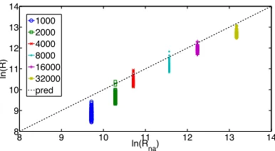
2 Critical Susceptibility for Strongly-Disordered Bosons in One Di-mension 44 2.1 Introduction . . . 44
2.2 Model . . . 48
2.3 Methodology: SDRG for the Disordered Rotor Model . . . 52
2.6 Conclusion . . . 86
3 Mott Glass to Superfluid Transition for Dirty Bosons in Two Di-mensions 88 3.1 Introduction . . . 88
3.2 Methodology: Numerical Application of the SDRG . . . 93
3.3 Numerical Results . . . 102
3.4 Phases and Quantum Phase Transitions . . . 130
3.5 Conclusion . . . 148
3.A Sum Rule vs. Maximum Rule . . . 155
3.B Measuring Physical Properties in the RG . . . 156
3.C The Pi(U) Gaussian, Pi(J) Power Law Data Set . . . 162
3.D Arguments for the Use of the SDRG in a Finite-Disorder Context . . 164
4 Many-Body Localization in a Quasiperiodic System 178 4.1 Introduction . . . 178
4.2 Model and Methodology . . . 183
4.3 Numerical Results . . . 188
4.4 Modeling the Many-Body Ergodic and Localized Phases . . . 202
4.5 Tracing the Phase Boundary . . . 210
4.6 Conclusion . . . 212
4.A Exact Diagonalization . . . 214
Chapter 1
Introduction
1.1
Noninteracting Particles in Perfect Media
The most basic theories of many-body and solid-state physics treat
noninteract-ing particles propagatnoninteract-ing in perfectly periodic environments (e.g., electrons in crystal
lattices). This thesis concerns situations in which this picture fails completely. More
precisely, it examines physical systems where particle-particle interactions and
ape-riodicity (e.g., disorder) combine to lead to novel phenomena. Before delving into
the effects of these two ingredients, it is useful to revisit the simplified theories that
ignore them and recall their successes and inadequacies1.
1.1.1
Electrons in a Metal as an Ideal Fermi Gas
In 1900, Drude formulated the first model of conduction in metals by considering
a classical gas of conduction electrons moving in a static background of positive ions.
He assumed that electrons propagate freely between collisions with the ionic
back-1Readers who are familiar with the important roles that disorder and interactions individually
ground, that each electron’s collisions are typically separated by a mean scattering
time τ, and that the electrons emerge from these scattering events with velocities obeying the classical Maxwell-Boltzmann distribution. Using these assumptions, he
was able to make predictions for certain quantities that roughly match
experimen-tal observations. Nevertheless, other measurements deviated strongly from Drude’s
predictions. Most notably, experimental values of the specific heat cv did not show the classically expected value of 3
2kB per conduction electron. This particular
defi-ciency was remedied in the early years of quantum mechanics by Sommerfeld, who
replaced the Maxwell-Boltzmann distribution in Drude theory with the Fermi-Dirac
distribution for the occupation of a single-particle state of energy E:
fFD(E) =
1
eE
−µ kBT + 1
(1.1)
Nevertheless, several quantitative and qualitative mysteries remained. Most
funda-mentally, the theories of Drude and Sommerfeld failed to explain why some solid-state
materials are nonmetallic [12].
To begin to classify materials as metals and insulators, it was necessary to treat
the positive ions of Drude and Sommerfeld’s theories more carefully. X-ray
diffrac-tion experiments suggested that these ions are often arranged in periodic lattices,
motivating the study of the quantum mechanics of a particle in a perfectly periodic
potential:
−~ 2
2m∇
Here,U(~r+R~) =U(~r), whereR~ is any of the elementary lattice vectors that translate the lattice into itself. The eigenstates of this problem satisfy Bloch’s theorem:
ψn,k(~r+R~) = ei~k· ~ Rψ
n,k(~r) (1.3)
where~k is a vector within the unit cell of the reciprocal lattice defined by ei ~K·R~ = 1 (known as thefirst Brillouin zone). Bloch’s theorem allows us to solve the Schr¨odinger
equation within a single unit cell, because up to a phase, the eigenstates are
peri-odic between unit cells. The eigenenergies En(~k) typically segregate into a series of bands, labeled by the index n, separated by energetic band gaps. In the case of the Schr¨odinger equation (1.2), there are an infinite number of bands, corresponding to
the discrete, but infinite, solutions within a unit cell. An example for a particles in a
weak periodic potential is shown in Figure 1.1.
Often, the problem is simplified further by making thetight-binding approximation
that there are only a fixed number of orbitals that a particle can occupy within each
unit cell:
ˆ
Htb =J L X
j=1
(ˆc†j+1cˆj+ ˆc†jˆcj+1)− L X
j=1
µjnˆj (1.4)
If the potential µj repeats every n lattice sites, then there is an n-site unit cell, and correspondingly, there will be n bands. In this tight-binding approximation, Bloch’s theorem guarantees that the eigenstates will be periodic (again, up to a phase) each
n sites.
k
E
⇡ a ⇡
a
2
U
[image:14.612.241.406.75.266.2]2
U
Figure 1.1: The energyE vs. quasimomentumkfor particles in 1D in a weak periodic potential of period a and strength U. The quadratic dispersion for a free particle is folded into the first Brillouin zone, and degenerate states whose quasimomenta differ by an integer number of reciprocal lattice vectors get split by the potential. This induces band gaps of size 2U.
values of electronic spin. Suppose there is an odd number of conduction electrons
per unit cell. Then, in the ground state, the highest occupied band will only be half
filled. In the limit of an infinitely large system, there will be no energetic barrier to
adding another electron. In other words, the Fermi energy EF lies in the conduction
band, and the material conducts at low temperatures. Alternatively, suppose there
is an even number of conduction electrons per unit cell. Then, the highest occupied
band is fully filled, and it is necessary to pay the energetic cost of the band gap to add
another electron. Therefore, EF lies in a band gap, and the system is an insulator at low temperatures. This forms the most basic band classification of solid-state
1.1.2
Bose-Einstein Condensation
In parallel with these studies of the properties of solid-state materials, the
obser-vation of viscosity-free flow in liquid helium at low temperatures motivated the study
of systems composed of many bosons. The occupation of single-particle energy levels
by bosons is described the Bose-Einstein distribution:
fBE(E) =
1
eE
−µ kBT −1
(1.5)
Meanwhile, the density of states of an ideal gas scales like ρ(E) ∼ Ed−22. Einstein noted that, in three dimensions and at low enough temperature, there is a bound to
the number of particles that can be accommodated in excited single-particle states.
Hence, there will be a macroscopic accumulation of bosons in the single-particle
ground state, a phenomenon now known as Bose-Einstein condensation [48]. The
ground state condensate can be thought of as a single coherent quantum state with
an overall number and phase.
Important experimental properties of helium-4 deviate from the predictions for
the ideal Bose gas. For instance, helium-4 has a divergence in the specific heat
at the transition to the so-called superfluid state instead of a cusp at the
Bose-Einstein condensation temperature [62]. Furthermore, superfluidity can occur in two
dimensions [83, 40]. Nevertheless, the ideal Bose gas treatment gives a rough estimate
of the transition temperature in helium-4 and was recognized as being the conceptual
1.2
The Role of Interactions
1.2.1
From Fermi gases to Fermi liquids
At least in the case of electrons in metals, it may seem like a miracle that the band
theory picture is ever useful. After all, electrons interact strongly through Coulomb
forces. Indeed, the typical Coulomb energy per particle in a good metal is typically
three to five times the Fermi energy [42]. Why then is an independent electron picture
often applicable?
Landau answered this question by arguing that there are indeed entities that can
be treated as independent in a metal, but that these are not the bare electrons.
In-stead, in Landau’s Fermi Liquid Theory, the bare electrons effectively get “dressed”
by weak interactions, giving rise to emergent quasiparticles. These quasiparticles are
in one-to-one correspondence with the bare electrons and are therefore also described
by Fermi-Dirac statistics. However, these quasiparticles are effectively free (i.e.,
non-interacting). Landau showed that these emergent particles are stable to
quasiparticle-quasiparticle scattering, due to the difficulty of constructing momentum-conserving
scattering events with particles near the effective Fermi surface. Thus, the difference
between the noninteracting and interacting electron systems could be encapsulated in
a few renormalized parameters describing the quasiparticles (e.g., an effective
quasi-particle massm∗ that differs from the bare electron massm
e) [12]. Figure 1.2 shows
the ground state momentum occupation function in a Fermi Liquid. In terms of the
mo-k
f
F D(
k
)
1
k
FZ
Figure 1.2: The ground state momentum occupation for noninteracting fermions (blue dashed line) and for a Fermi liquid (red solid line). In terms of the bare electrons, there is some filling of momenta beyond the Fermi wavenumber kF, but there is a relic of the step function occupation in the noninteracting system (the “quasiparticle residue,” here called Z). This feature is a reflection of the fact that the momentum occupation in terms of quasiparticles is indeed that of a noninteracting system.
mentum kF of the non-interacting problem; however, in terms of quasiparticles, only momenta up tokF are filled.
1.2.2
From Bose-Einstein Condensates to Superfluidity
To explain the discrepancies between experimental observations on helium-4 and
Bose-Einstein condensation, it was also necessary to study the role of interactions
in many-boson systems. Bogoliubov introduced weak interactions to a Bose gas and
showed that excitations on top of the Bose-Einstein condensate obey a linear
dis-persion ω~k ∼ |~k| at small wavevector |~k| [26]. Then, it was possible to invoke an argument by Landau that, to preserve energy and momentum conservation, the
con-densate cannot exchange energy with its environment through low-energy processes
Eventually, the interacting Bose gas picture was also recognized as being
inti-mately related to superconductivity and to superfluidity in helium-3. Electrons and
helium-3 atoms are both fermions; thus, for a superfluid to form, a mechanism is
required to “pair” these fermions into effective bosons. In ordinary superconductors,
this is due to effective attractive electron-electron interactions mediated by phononic
modes of the lattice [33, 16]. In helium-3, the pairing mechanism instead involves
magnetic interactions between atoms of the same spin [62, 91].
1.2.3
Fundamental Failures of Noninteracting Models
We have seen above that, for sometimes rather subtle reasons, noninteracting
models can provide useful starting points for the study of weaklyinteracting systems
of bosons and fermions. There are circumstances, however, where noninteracting
pictures fail completely. We will now discuss two such situations.
1.2.3.1 The Tomonaga-Luttinger Liquid in One Dimension
For instance, consider the low temperature properties of fermions in one spatial
dimension. Here, no finite interaction strength can truly be considered weak. The
Fermi surface in one dimension consists of only two points at ±kF. These degenerate states will be split by even weak interactions, destroying the entire Fermi surface and
rendering the Fermi Liquid Theory inapplicable [139].
Tomonaga realized that the emergent “particles” in one dimension are not the
quasiparticles of Fermi Liquid Theory but rather collective bosonic modes. He used
these modes:
ˆ
Hb = u
2π Z
dx
1
K(πΠφ)
2+K(∂ xφ)2
(1.6)
The Hamiltonian (1.6) represents the case of spinless fermions, and the bosonic
op-erators ˆφ and ˆΠφ obey [ ˆφ(x),Πˆφ(x0)] = iδ(x−x0). The parameter K depends on the microscopic interactions: K < 1 corresponds to attractive interactions, K = 1 corresponds to noninteracting fermions, and K >1 corresponds to repulsive interac-tions [136]. Luttinger calculated the ground state momentum distribution and showed
that it is a power law that depends on K [97]. This is in contrast to the occupation function for a Fermi Liquid in Figure 1.2.
Later, Haldane realized that the model (1.6) is much more generally applicable
to one-dimensional systems. In particular, it can also be applied to repulsively
inter-acting bosons, but the relationship of K to the microscopic interactions is different:
K = ∞ corresponds to the noninteracting limit, and K decreases with interaction strength [64].
1.2.3.2 The Mott Insulator
There is another fundamental limitation of noninteracting models that applies in
arbitrary dimensions: the Fermi and Tomonaga-Luttinger Liquid Theories can break
down at nonperturbative interaction strengths. Landau’s argument, for example,
relies on an adiabatic continuity between the bare electrons of the truly noninteracting
model and the quasiparticles of the weakly interacting model [12]. It is important to
In fact, when Fermi Liquid Theory was proposed, experiments had already shown
that there are insulating materials that band theory incorrectly classifies as
con-ductors. Classic examples are the transition metal oxides with an odd number of
electrons per unit cell (e.g.,V2O3). Since these materials often exhibit
antiferromag-netism at low temperatures, Slater proposed that the unit cell gets “doubled” due to
the spin structure. Then, the insulating behavior would still follow from band
the-ory since there would now be an even number of particles per unit cell. There was,
however, a problem of scales: the antiferromagnetic ordering does not set in until
T ∼ 102K while the insulating behavior can persist until much higher temperatures
of the order T ∼ 103 −104K [42]. This motivated Mott to look outside the band
theoretic paradigm for an explanation for the insulating behavior. He reasoned that
electrons cannot be mobile if they do not have enough kinetic energy to overcome
strong electron-electron Coulomb repulsion. Instead, the electrons get localized in a
particular unit cell, forming an insulating state known as the Mott insulator [105].
Each localized electron still carries a spin degree of freedom, and these spins can
order at low temperatures, giving rise to the antiferromagnetic ground state. Thus,
the insulating state sets the stage for the spin ordering and not vice versa [42].
Although motivated by the inadequacies of band theory in describing certain
elec-tronic systems, Mott’s argument is clearly not restricted to fermions. Many-boson
systems can also transition from the superfluid state to a Mott insulating state at
strong interaction strengths, and we will now proceed to discuss models that can
1.2.4
The Fermi and Bose Hubbard Models
A minimal model for studying the role of interactions in electronic systems is the
Fermi-Hubbard model:
ˆ
HFH =J X
hj,ki,σ
(ˆc†j,σˆck,σ+ ˆc†k,σcˆj,σ) +U X
j ˆ
nj,↑nˆj,↓ −µ
X j,σ
ˆ
nj,σ (1.7)
Here, we introduce on-site interactions between electrons to a tight-binding model
(1.4) with a single-site unit cell. The operators ˆcj and ˆc†j obey the fermionic anti-commutation relation {ˆcj,ˆc†k}=δj,k and the number operator ˆnj = ˆc†jˆcj. The ground state of the one-dimensional model at half-filling (i.e., one particle per unit cell) was
obtained by Lieb and Wu, who showed that there is no conducting state for U > 0 [93]. In higher dimensions, no such exact solution has been found, and the
Fermi-Hubbard model has inspired decades of numerical and theoretical work. The relevance
of this model to the high-temperature superconductors and heavy fermion materials
has especially motivated efforts to understand its phase diagram.
A somewhat simpler2 variant of the Fermi-Hubbard model is the Bose-Hubbard
model, where the particles hopping on the lattice are (typically spinless) bosons:
ˆ
HBH =J X
hj,ki
(ˆb†jˆbk+ ˆb†kˆbj) +
U
2
X j
ˆ
nj(ˆnj−1)−µ X
j ˆ
nj (1.8)
Here, the operators ˆbj and ˆb†j obey the bosonic commutation relation [ˆbj,ˆb†k] = δj,k
2The Bose-Hubbard model is simpler because it is amenable to quantum Monte Carlo, while
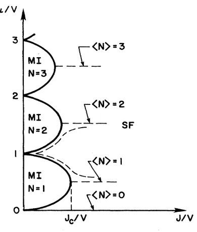
and the number operator ˆnj = ˆb†jˆbj. The ground state phase structure of this model was studied in the late 1980s by Fisher, Weichman, Grinstein, and Fisher and is
shown in Figure 1.3 [55]. These authors began by examining the model at zero
hopping strength, J = 0. Here, the model is trivially insulating with a fixed density of bosons per site that is determined by minimizing U2n(n−1)−µn. As the hopping is raised, isolated boson-hole pairs are added on top of this inert background, but the
overall density stays fixed. There remains a finite gap to the addition of single bosons
or holes, and the system remains a Mott insulator. The transition to superfluity
generically occurs when the gap to the addition of single bosons or holes closes, and
then, any additional particles added to the system propagate freely on top of the
inert background. This determines the general phase structure seen in Figure 1.3,
with “Mott lobes” at small hopping. The superfluid-insulator transition takes on a
special character at the tip of each lobe, where there is an emergent particle-hole
symmetry. For this reason, the overall density of bosons stays fixed even after exiting
the Mott lobe, and the ground state instead becomes a superposition of different ways
to redistribute the same density around the system [55].
1.3
Aperiodicity and Localization
We have seen above that strong interactions can drive otherwise metallic or even
superfluid systems into a Mott insulating state. There is another distinct route to
insulating behavior that does not require interactions. To understand this mechanism,
BOSON LOCALIZATION AND THE SUPERFLUID-INSULATOR. .
.
quence
of
the competition between the kinetic energy, which tries to delocalize the particles and reduce thephase fiuctuations
of
the Bose field, and the combinationof
the interactions and the random potential which try tolocalize the particles and make the number density Auc-tuations small. This competition plays an essential role
in the scaling analysis
of
the superAuid onset transitionwhich was briefiy introduced in Ref. 3 and is discussed in
more detail here.
In this paper we discuss the behavior
of
bosons withshort-range repulsive interactions moving in both ran-dom and periodic external potentials. We argue that, in general, there can be three types
of
phases at zerotem-perature: a superAuid phase, commensurate Mott insu-lating phases in which there is a gap for particle-hole ex-citations and zero compressibility, and a
"Bose
glass"phase in which there is no gap, the compressibility is finite, but the system is an insulator because
of
the locali-zation eft'ectsof
the random potential. This Bose glassphase, which is rather analogous to the Fermi glass phase
of
interacting fermions in a strongly disordered potential,with the repulsive interactions playing the role
of
Pauliexclusion, has some rather surprising properties,
particu-larly an infinite superAuid susceptibility. The principal
focus
of
this paper is the onsetof
superQuidity at zero temperature as the parametersof
the system are varied.Two groups have recently studied the onset
of
superAuidity in a random potential. Ma, Halperin, and
Lee (MHL) have attempted a Landau theory and dimen-sionality expansion about a mean-field theory; we believe (and will argue) that this work contains an error which invalidates the conclusions. Giamarchi and Schulz, on
the other hand, have analyzed the interacting Bose
prob-lem in one dimension by a renormalization-group calcula-tion perturbacalcula-tion in the strength
of
the disorder. We willrely heavily on this calculation as a cornerstone on which
to test more general scaling arguments.
We will argue that, in contrast to natural expectations, the onset
of
superfiuidity at zero temperature is generallynot in the universality class
of
the 0+1-dimensionalXY
model (with, in the presence
of
randomness, a random time-independent potential). Instead, we will show thatin the absence
of
randomness, such 4+1-dimensionalXY
models describe only special multicritical transitions
while generically the behavior is that
of
a zero-densitytransition such as that which occurs as the density
of
bo-sons is increased from zero in the absenceof
an external potential. (This is also the case for the generic quan-tumXY
magnet without time reversal invariance. ) In the presenceof
randomness, we expect the transition tosuperAuidity always to occur from the Bose glass phase. This transition, as argued in Ref. 3,is characterized by a dynamic critical exponent z which because
of
number-phase competition turns out to be equal to the spatial di-mension d, a correlation length exponentv~
2/d, and anorder-parameter exponent
g.
This latter exponent isar-gued here to satisfy the bound g
~
2—
d. These exponentrelations, when placed in the framework
of
a scalingtheory, enable explicit and verifiable predictions for
vari-ous static and dynamic properties near the
zero-temperature superfluid onset transition. Some
measur-able exponents, depending only on z, are predicted
exact-ly.
We present arguments that there may, in fact, be no
simple high-dimensional limit
of
this transition—
at leastnot
of
a conventional G-aussian or mean-field kind—
andthat the equality z
=d
holds in all dimensions. We alsooutline an alternate possibility, discussed by Weichman
and Kim in Ref. 8, that for
d)
4 there are two universali-ty classes, one for strong disorder with presumably z=d
and the other for weak disorder with mean-field ex-ponents.
The outline
of
this paper is as follows: In Sec.II
the basic modelof
bosons hopping on a lattice is introduced.Its relation to the usual charging models
of
granular superconductivity'
is brieAy explained. By treating the kinetic energy (i.e., hopping) as a perturbation, the phasediagram in the hopping strength,
J,
and chemical poten-tial,p,
plane is worked out.For
the pure, nonrandom, system we find two typesof
phases: a setof
incompressi-ble Mott insulating phases in which the density is fixed commensurately at a positive integer, n, per site; and a
superAuid phase with the usual ofMiagonal long-range
order (Fig. 1). In the random case we argue that a gap-less, insulating Bose glass phase with nonzero
compressi-bility, must intervene between the Mott and superAuid
phases (Fig. 2), and that, in fact, the Mott phase can be
destroyed completely if the randomness is su%ciently
strong (this is almost certainly the relevant case for the phase diagram
of
He adsorbed in porous media). InAp-pendix A we derive the exact phase diagrams within a
mean-field theory (i.e., an infinite-range hopping model), verifying many
of
the general details, but finding no Boseglass phase. This, however, is hardly surprising since lo-calization e6'ects are absent when hopping can occur
be-tween any two sites, particularly those with degenerate onsite energy.
yQN0'=0
J
/V [image:23.612.225.420.77.306.2]FIG. 1. Zero-temperature phase diagram for the lattice mod-el ofinteracting bosons, (2.1),in the absence ofdisorder. For an integer number ofbosons per site the superAuid phase (SF) is unstable to a Mott insulating (MI) phase at small
J/V.
Figure 1.3: The general phase structure of the Bose-Hubbard model (1.8), as worked out by Fisher, Weichman, Grinstein, and Fisher [55]. Note that V in their phase diagram is the interaction strength that we call U in our definition of the Bose-Hubbard model (1.8).
1.3.1
Anderson Localization
In 1958, Anderson was motivated by Feher’s experiments on spin diffusion in
silicon to examine the role of disorder in quantum transport [11]. He studied a
tight-binding single-particle model of the form (1.4) where µj varies randomly from site to site. Anderson sampled the µj randomly from a box distributions of width W. This serves as a toy model of the situation in real materials where the environment
(e.g., a crystalline lattice) is never perfect: impurities and structural imperfections
are inevitable. Anderson showed that, below some ratio of the hopping to the disorder
strength, the single-particle eigenstates will all be localized. This means that their
amplitude decays exponentially in space with a characteristic lengthξ, thelocalization
systems where Bloch’s theorem holds. Soon thereafter, Mott and Twose argued that
all eigenstates will be localized in one spatial dimension for arbitrarily weak disorder
in the potential [107]. This reveals an important aspect of Anderson localization:
it occurs even when J >> W, meaning that the kinetic energy is great enough to surmount any barriers imposed by the potential. Anderson localization is thus not
due to any form of classical trapping and is instead a wave interference phenomenon.
In 1979, the nature of Anderson localization in higher dimensions was clarified
by Abrahams, Anderson, Licciardello, and Ramakrishnan [2], who built on earlier
ideas of Thouless and collaborators [45, 135, 92]. These authors formulated a scaling
theory of localization by considering how the conductance g varies with the linear system size Lin dimension d. At small disorder strength, the conductance should be ohmic:
g(L)∼Ld−2 (1.9)
Meanwhile, at strong disorder, localization implies that the conductance decays
ex-ponentially with L:
g(L)∼exp
−L
ξ
(1.10)
Abrahams et al. examined the function:
β(g)≡ dlng
dlnL (1.11)
which describes how the conductance varies as the system size is changed. The goal
Figure 1.4: The beta function vs. conductance g, as derived in the paper by Abrahams et al. [2].
possible to extract a picture like the one in Figure 1.4. In one dimension, the β
function (1.11) is always negative, indicating that the system flows towards lower and
lower conductances as the sample size is raised. This is consistent with the notion that
that one-dimensional disordered systems are always localized. In three dimensions,
the β function crosses zero at some finite value of the conductance g. This indicates that the presence of an Anderson transition between localized and ohmic behavior.
The case of two dimensions is marginal, because the level of analysis in equation
(1.9) suggests that the ohmic conductance is independent of system size. Thus, the
sign of the β function is determined by logarithmic corrections to equation (1.9). Abrahams et al. showed that this correction is typically negative, meaning that the
two-dimensional model is always localized3 [2].
Let us now focus on the nature of the Anderson transition in three dimensions.
Figure 1.5 shows a caricature of the density of states of the three-dimensional
⇢
(
E
)
E
localized) localized)
extended)
mobility) edges)
Figure 1.5: Sketch of the density of states of the three-dimensional Anderson model. Mobility edges separate the localized and extended states in the spectrum.
derson model. Whereas in one and two dimensions the entire spectrum would be
localized, here extended and localized states can coexist. However, they generally
cannot coexist at the same energy: as argued by Mott, if there were degenerate
ex-tended and localized states, they would be strongly mixed by small perturbations.
This mixing would render both states extended [108]. Consequently, localized and
extended states are typically separated by so-calledmobility edges, as shown in Figure
1.54. For a system of electrons, the conductance properties will be determined by the
location of the Fermi energy (i.e., whetherEF lies in a region of localized or extended
states). The Anderson transition can be tuned by changing the disorder strength,
thus moving the mobility edge past EF. Alternatively, the transition can be tuned
by changing the number of electrons in the system at fixed disorder strength, thus
tuning EF past the mobility edge.
The scaling theory (as presented in Figure 1.4), suggests that the conductance
4At sufficiently strong disorder strength, the entire spectrum can be localized even in three
will go to zero as we approach the thermodynamic limit in a localized regime. In real
solid-state systems, it is important to remember that the electrons interact with a
phononic bath. By absorbing and emitting phonons, electrons can hop between
dis-tant localized orbitals. The probability of such an event depends upon the splitting in
energy between the orbitals (i.e., hopping is more favored between nearly degenerate
states) and on the distance separating the orbitals, because the overlap of the orbital
wavefunctions decays exponentially in space. Mott determined how to balance these
effects and thereby obtained the variable-range hopping conductivity:
σ ∝exp
" −
T0
T 1
d+1#
(1.12)
in d dimensions. Here, T is the temperature of the phononic bath, and T0 is a
characteristic temperature related to the typical energy splitting of orbitals within
a localization volume ξd [106]. The variable-range hopping process is ultimately responsible for bringing the electrons into thermal equilibrium with the phononic
bath. The problem of many-body localization, which we will discuss in Section 1.4.2.2
below, is intimately tied to the question of whether electron-electron interactions can
1.3.2
Other Models of Localization
1.3.2.1 Localization with Hopping Disorder
Localization is a general wave phenomenon that occurs in many disordered
quan-tum systems; it is not special to the model studied by Anderson. For instance,
localization also occurs with “off-diagonal” disorder in the hopping term:
ˆ
Hrh =− L X
j=1
Jj(ˆc†j+1ˆcj + ˆc†jcˆj+1) (1.13)
This one-dimensional random hopping model has a particle-hole symmetry that is
missing in the Anderson model. The related classical problem of the random harmonic
chain was studied in the early 1950s by Dyson [43], and the quantum model received
attention in the following decades [133, 46]. More recently, higher-dimensional
ver-sions of this model have been studied [103]. Furthermore, the model has been realized
experimentally in photonic waveguides [89], and there is also a proposal to engineer
it in atomic lattices [150].
Perhaps the most intriguing feature of the one-dimensional model is that all
eigen-states are localized except one: the E = 0 state. This can be shown by setting ˆ
Hrh|ψi= 0, which yields the equation:
−Jjψj+1−Jj−1ψj−1 = 0⇒ ψj+1 ψj−1
=−Jj−1
Jj
This in turn implies that the localization length ξ near E = 0 obeys:
1
ξ = −nlim→∞ 1 2nln
ψ2ψn1+1
= − lim
n→∞ 1
2n[(ln|J2n−1|+ ln|J2n−3|+· · ·+ ln|J1|)
−(ln|J2n|+ ln|J2n−2|+· · ·+ ln|J2|)] (1.15)
For uncorrelated disorder, the limit goes to zero. This means thatξ diverges, indicat-ing the presence of an extended zero energy state. As a function ofE, the localization length is known to diverge as ξ(E)∼ −ln|E| and this divergence is accompanied by a Dyson singularity ρ(E)∼ 1
|Eln3E| in the density of states [43, 133, 149].
1.3.2.2 Aubry-Andr´e Localization
A couple of decades after Anderson’s original work on localization, Aubry and
Andr´e demonstrated that localization can even occur without “true” disorder. They
studied a tight-binding model of the form:
ˆ
HAA =J X
j
(ˆc†j+1ˆcj+ ˆc†jˆcj+1) +h X
j
cos (2πkj+δ)ˆnj (1.16)
with irrational wavevectork. This makes the potentialincommensurate with the lat-tice, which in turn means that the potential pattern is deterministic but nonrepeating
[13]. Harper had studied a similar model much earlier, but he had focused on a special
ratio of hopping to potential strength [65]. Aubry and Andr´e showed that this point
all single-particle eigenstates are extended, from a strong potential phase, where all
eigenstates are localized.
The easiest way of demonstrating that the transition exists is by noting that
the model (1.16) is self-dual when δ = 0. On a finite size lattice, it is conven-tional to enforce periodic boundary conditions by choosing k = L` such that ` and L
are mutually prime. The self-duality can be realized by switching to Fourier space
(cj = √1LPqeiqjcq) and then performing a rearrangement of the wavenumbersq such that the real-space potential term looks like a nearest-neighbor hopping in Fourier
space and vice versa. The duality construction reveals that, if the AA model has a
transition, it must occur at J h =
1
2. In the thermodynamic limit, there is indeed a
transition at this value for nearly all irrational wavenumbers k [134]. When Jh > 12, all single-particle eigenstates are spatially extended, and by duality, localized in
mo-mentum space; when J h <
1
2, all single-particle eigenstates are spatially localized, and
by duality, extended in momentum space. Exactly at Jh = 12, the eigenstates are
multifractal [127, 67]. The spatially extended phase of the AA model is characterized
by ballistic, not diffusive, transport [13]. Recently, Albert and Leboeuf have argued
that localization in the AA model is a fundamentally more classical phenomenon than
disorder-induced Anderson localization, and that the AA transition at g = 12 is most simply viewed as the classical trapping that occurs when the maximum eigenvalue of
the kinetic (or hopping) term crosses the amplitude of the incommensurate potential
[4].
local-ization transition for its own peculiarities and because it mimics the situation in
disordered systems in d ≥ 3, where there is also a single-particle localization tran-sition5 [134, 30, 49, 1, 47, 127, 67, 138]. It is important to keep in mind that, in
contrast to the three-dimensional Anderson model, the Aubry-Andr´e model (1.16)
lacks a mobility edge. However, a mobility edge is introduced by many perturbations
to the model (1.16) [116].
1.4
Disorder, Interactions, and Phase Transitions
We have seen above that interactions and disorder can both localize particles,
leading to Mott and Anderson insulators respectively. We might, consequently, be
led to believe that the combination of both ingredients would favor insulating behavior
even more strongly. This naive assumption underestimates the considerable richness
of the disordered many-body problem. Interactions can destroy disorder-induced
localization, and disorder can transform Mott insulators into exotic glassy states. We
will now discuss these fascinating phenomena. We will first address some general
aspects of the role of disorder at and near phase transitions; then, we will concretize
these ideas to two issues of special relevance to this thesis.
5The AA model was also actively investigated in the mathematical physics literature, because it
1.4.1
Disorder at Phase Transitions
1.4.1.1 The Harris Criterion
Suppose we introduce disorder into a system that exhibits a continuous phase
transition in the clean limit. Two questions immediately arise: does a sharp transition
survive the presence of disorder, and if so, how do the universal properties of the
transition change? In 1974, Harris formulated a general criterion that can guide
the effort to address these questions. Harris originally formulated his argument in
the context of thermal phase transitions tuned by the temperature. Here, we use
the thermodynamic language for convenience, but Harris’ argument applies equally
well to a quantum phase transition tuned by some other parameter. At the clean
transition, the correlation lengthξdiverges as |T−Tc|−ν. Meanwhile, in a disordered system, there is actually a “local” critical temperature Tc,loc that varies spatially,
because of local variations in the couplings. To maintain the integrity of the clean
critical point, the typical fluctuation of Tc,loc in a correlation volume ξd ought to be
smaller than the distance to criticality |T −Tc|. The central limit theorem suggests that fluctuations of the mean of Tc,loc in a localization volume decay as ξ−
d
2. Thus,
we require:
ξ−d2 =|T −Tc|−dν2 <|T −Tc| (1.17)
This yields an inequality, the Harris criterion, that must be obeyed by the critical
point of any disordered system:
If a clean critical point obeys the condition (1.18), then the universal properties will
be unaffected by introducing weak disorder. Alternatively, if the clean critical point
violates the condition, there are two possibilities: weak disorder may completely smear
the transition away, or a critical point with new universality may emerge [66, 120].
1.4.1.2 Griffiths Phases and Rare Events
Let us consider the case where a transition survives in the disordered system.
Irrespective of whether or not the universality changes, there will be consequences
for the phases that the transition separates. We label these abstract phases A and
B. Due to the spatial variation in the couplings, when the bulk of the system is in
phase B, there can still be regions that are locally in phase A, as shown in Figure
1.6. These regions are known asGriffiths regions, and the phase in which they appear
is known as a Griffiths phase. If the disorder is spatially uncorrelated, the Griffiths
regions get exponentially rare as their size increases. Nevertheless, arbitrarily large
Griffiths regions can appear [61, 140].
Pollet et al. have recently argued that Griffiths regions exclude the possibility
of standard phase transitions between energetically gapped and gapless phases in
disordered systems. As we approach the transition from the side that is gapped in
the clean system, there will appear arbitrarily large regions of the competing gapless
phase, driving the system gapless [113]. According to Pollet et al., any transition
between gapped and gapless phases in a disordered system must be of the “Griffiths
al-B"
A
A
A
B"
Figure 1.6: Schematic depiction of a Griffiths phase in a disordered system. The bulk of the system is in phase B, a gapped phase of the clean system. However, there are regions that are locally in the phase A, and these regions can get arbitrarily large in the thermodynamic limit. Since phase A is gapless, the Griffiths phase will also be gapless due to the presence of these rare regions.
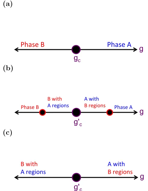
suppose phases A and B are gapless and gapped phases of the clean system
respec-tively, as shown in panel (a) of Figure 1.7. In the disordered system, two Griffiths
phases will flank the “true” phase transition. This situation is shown in panel (b).
Both Griffiths phases will be gapless, so the only transition between gapped and
gapless phases is the transition out of the pure phase B, which is indeed of Griffiths
type. Note that, if the disorder distributions are unbounded, it is always possible
to find regions of the competing phase, so the gapped phase B will, presumably, be
completely destroyed, as in panel (c) of Figure 1.7 [63].
Griffiths regions are examples of rare events in disordered systems, and these
rare events can lead to very unusual behavior: average values of physical properties
can behave very differently from their typical values. An instructive example was
found by Fisher, who studied the paramagnet-ferromagnet phase transition of the
(a)
Phase"B" Phase"A"
gc
g
(b)
B"with"
A"regions"
Phase"B"
g'c
g
Phase"A" A"with"
B"regions"
(c)
B"with"
[image:35.612.200.445.171.487.2]A"regions" A"with"B"regions" g g'c
function hσˆz
jˆσjz+ri in the paramagnetic phase, and showed that the typical and mean correlations both decay exponentially. However, the correlation lengths over which
these decay occur are very different, because the mean correlation at large distances
is dominated by exponentially rare pairs that are perfectly correlated [54].
1.4.1.3 Infinite-Disorder Fixed Points and the Strong-Disorder
Renor-malization Group
The most extreme impact of disorder upon phase transitions occurs when a system
exhibits a so-called infinite-disorder fixed point. These special fixed points are often
identified through a powerful technique for studying strongly disordered systems, the
strong-disorder renormalization group(SDRG). This method was originally developed
by Dasgupta and Ma [37] and Bhatt and Lee [22]. Later, it was used extensively by
Fisher to study a variety of one-dimensional quantum spin models [52, 54].
One way to motivate the procedure is to note that strong disorder makes the
problem of finding the quantum ground state of a model more local. Having identified
the strongest of all the disordered couplings in the Hamiltonian, we can then use the
assumption of strong disorder to argue that other couplings in the real-space vicinity
of this coupling are likely to be much weaker. This means that the ground state can
locally be approximated by satisfying just this dominant coupling. Other terms in the
Hamiltonian can then be incorporated as corrections6. This procedure generates new
effective couplings in the model and thereby yields a new effective Hamiltonian. Since
6Quite often, these other terms are treated by means of perturbation theory, but this need not
part of the ground state is specified in this step, some degrees of freedom of the system
are decimated away. By repeating the procedure, we can iteratively specify the entire
ground state [37, 22]. Moreover, we can examine the way in which the probability
distributions of the disordered couplings flow as the renormalization proceeds. One
possibility is that the model looks more and more disordered at larger length scales
near criticality, thus flowing towards “infinite disorder.” If this occurs, the strong
disorder renormalization group becomes asymptotically exact near criticality, and it
is sometimes even possible to predict quantities for which the corresponding behavior
in the clean model is unknown [52, 53].
Fisher used the SDRG to show that several one-dimensional quantum spin models
exhibit this type of fixed point. These include the random transverse-field Ising chain
and various random antiferromagnets [52, 54]. Numerical work by Motrunich et al.
subsequently provided evidence that infinite-disorder criticality also characterizes the
two-dimensional random transverse-field Ising model [104]. The discrepancy between
typical and mean values is most dramatic at infinite-disorder criticality. Again, a
striking example was found by Fisher: in the random transverse-field Ising chain, the
typical two-point correlations at criticality obey lnhσˆz
jσˆzj+ri ∼ − √
x while the mean two-point correlations obey hσˆz
jσˆjz+ri ∼ x21−φ where φ =
√
5−1
2 is the golden mean.
Since the latter is what is measured in neutron-scattering experiments, it is crucial to
keep this distinction between mean and typical values in mind when confronted with
1.4.2
The Disordered, Interacting Many-Body Problem
We will now focus on two challenging problems of current theoretical and
experi-mental interest: the dirty boson and many-body localization problems. In both cases,
the interplay of disorder and interactions is absolutely crucial for characterizing the
phases and phase transitions, but the inherent difficulty of each problem has left a
full understanding elusive.
1.4.2.1 Superfluid-Insulator Transition for Disordered Bosons
In the 1980s, seminal experiments on helium adsorbed in Vycor first attracted
the attention of theorists to the “dirty” or random boson problem [35, 115]. These
experiments seemed to show a superfluid-insulator transition with some striking
sim-ilarities to ideal Bose gas behavior7. Thus, in the decade before the realization of
Bose-Einstein condensation in cold atomic gases, the helium in Vycor system was
ac-tually proposed as a possible realization of this elusive phenomenon. While studies of
disordered bosons did not ultimately lead to the observation of Bose-Einstein
conden-sation, the considerable richness of the dirty boson problem continued to stimulate
theoretical interest.
Both this richness and the difficulty of the dirty boson problem originate in the
volatility of the combination of disorder, interactions, and Bose statistics at low
tem-peratures. The single-particle ground state in a disordered potential is generically
localized [11]. The protocol for constructing the ground state of many noninteracting
7The most important similarity was the vanishing of the superfluid densityρ
s∼ |T−Tc|v near
criticality. In particular, a crossover from the interacting exponent of v = 2
3 to the ideal Bose gas
bosons is to simply deposit all of them in this localized state, but such a configuration
is intrinsically unstable to weak interactions. Thus, the noninteracting, disordered
limit is pathological and cannot be the starting point for a perturbative analysis.
Instead, Giamarchi and Schulz pioneered the study of dirty bosons in one
di-mension by introducing weak disorder to a strongly interacting many-boson system
[58]. The starting point of their analysis was a Hamiltonian of the form (1.6).
Gia-marchi and Schulz added a perturbative term describing a disordered potential and
decomposed it into terms describing forward and backward scattering by impurities.
They showed that the backward scattering leads to renormalization of the Luttinger
parameter K and disorder strength D. Their proposed renormalization group flow diagram is shown in Figure 1.8. The superfluid-insulator transition is described by
a fixed point at a universal value of the Luttinger parameter and vanishing
disor-der strength. For generic systems, the universal Luttinger parameter at criticality
is K = 32, and for particle-hole symmetric systems, it is K = 2. In either case, the transition is of Kosterlitz-Thouless type, meaning that superfluidity is destroyed by
the proliferation of phase slips in the superfluid order parameter [83]. Disorder is
dangerously irrelevant at the transition, because on the insulating side, the disorder
strength grows under renormalization. Unfortunately, when this occurs, the
perturba-tive approach of Giamarchi and Schulz breaks down and the insulating phase cannot
be characterized [58].
The task of identifying the insulating phase was taken up by Fisher, Weichman,
334 T.GIAMARCHI AND H.
J.
SCHULZ 37V.
I.
GCAI.IZATION TRANSITIONIXW OXK-DIMKXSIOX+r.
BQSGN SYSTEM
The method developed here can be applied to a
one-dln1enslonal system of 1Ilteractlng bosons 1Il a randonl
potential, and speci6cally to the localized-super Quid
transition in such a system.
%e
use a representation ofboson operators in terms of phase fields introduced by
Haldane. ' The single-boson creation operator is written
RS
and ri and g are the parts
of
the random potential with Fourier components around q=0
and q =+2mpo, respec-tively. We will take for i) and g the same probabilitydistributions as in (2.10). A unitary transformation
which exchanges P and
0
[p(p)~ —
p (p) in Eq. (2.3)]turns the complete problem [Eqs. (5.4) and (5.8)], into
the one discussed in Sec.
II,
Eqs. (2.4) to (2.11)(or moreprecisely its spinless analogue). Following the same
route as before, we find the scaling equations
dK
+
(x)=[p(x)]'~
e'~'"' (5.1) (5.10)1 BO(x)
+"
p(x)
=
—
g
exp[2im 8(x)],
Bx (5.2)
where 88(x)/Bx
=n.
[pa+
II(x)],
pu is the averagedensi-ty, and
II(x)
obeys the canonical commutation relations,[P(x),
II(x)]=i5(
x—
x')
. (5.3)The 1ong-wavelength-low-energy properties are
de-scribed by the Hamiltonian, '
0
=
f
dx (uK)(mII)+
—
(B„P)
2m
E
(5.4)where from Galilean invariance one has /u(nK)=po/m, and muK =a/(m pu), where a is the compressibility.
Clearly, the excited states of H are sound waves with
phase velocity u, which from Eq. (5.1) are the phonon
modes typical
of
a Bose superAuid. As already pointedout in the preceding section, the existence ofsuch modes
is suScient for true superAuidity to exist. ' The
coeNcient
E
determines the asymptotic behavior of thecorrelation functions,
(p(r)p(0)
)=
—
(2~por)where
p(x)
is the particle-density operator andP(x)
thephase of the boson field. Taking the discrete nature of
the particle density into account, the density operator is
where 2)=2)&/ir u 'po. Thus for K
~
—,'
the disorderscales to zero, indicating a delocalized, superAuid phase
with renormalized exponents due to the renormalization
of
E
ForE
p 3 the disorder grows under scaling,indi-cating that the properties of the system are qualitatively
di8'erent from the region
K
g —',. In analogy with theprevious chapter, we interpret this as the localized
re-gion. The phase diagram in the disorder EC plane is
shown in Fig. 5. Along the superAuid-localized transi-tion line, the fixed-point value
of
K
isE'
=-'„and
conse-quently the single-boson correlation function, Eq. (5.5)decays with a uniuersa/ power —, along this line. This is
the same exponent as found along the SS-PCD% limit
before. This equivalence certainly is not unexpected, as
in the SS region fermions are bound into singlet pairs,
with binding energy
5,
and these pairs behave likebo-sons, at least at large length scales.
The coefBcient K increases with increasing repulsion
between bosons
(K-x''
), and consequently thetransi-tion discussed above occurs with increasing repulsion.
In this context we may note than an external potential
with period 1/po (1 boson per site) is a relevant
pertur-bation, i.e., leads to a long-range ordered state, for
K
~
—,,i.
e., within the stable (against disorder) superfluidregion. On the other hand, a potential with period —,'po
(one boson per two sites) needs
K
y2
to lead to anor-dered state, and this can only be achieved for a very
strong repulsion with a finite range [5-function repulsion
leads to
K
&1 (Ref. 18)].+
Apu(pur) cos(2~par), (5.6)with son1e numerical constants A and
8.
%'e now introduce a random potential V, described by
an additional term
H„=
dxVxpx
(5.7)in the Hamiltonian. Inserting from (5.2) and retaining
only the most important terms (m
=0,
m=1),
thisbe-comes
Ja
/
r SUPSYFLU10 /
LOCAL12K0
a„=
I
dx[q(x)II(x)+[g(x)p,
e'""+H.
c.
]I,
(5.8)88(x)
=nil(x),
X (5.9)
where in
9
the linearly increasing part of8
is subtracted,FIG. 5. Phase diagrams for a one-dimensional boson system.
The thin lines indicate the qualitative shape of scaling
trajec-tories, as discussed in the text. The dashed lines are for parts
ofthe diagram that cannot be obtained by the present method.
[image:40.612.218.425.75.212.2]The Inulticritical point can also be located at I(
=0.
Figure 1.8: Renormalization group flows for weakly disordered bosons in one dimen-sion, as derived by Giamarchi and Schulz [58]. The superfluid-insulator transition is described by a fixed point at vanishing disorder strengthD. This transition separates a nearly uniform superfluid from an insulator in which the disorder strength grows with length scale, rendering the approach of Giamarchi and Schulz invalid.
dimension:
ˆ
HBH=J X
hj,ki
(ˆb†jˆbk+ ˆb†kˆbj) +
U
2
X j
ˆ
nj(ˆnj−1)− X
j
µjnˆj (1.19)
Their proposed phase diagram, as presented in a review by Weichman, is shown
in Figure 1.9 [146]. A Griffiths phase emerges and separates the Mott insulator
and superfluid in the phase diagram. This phase is globally insulating but contains
arbitrarily large regions of superfluid ordering. Thus, the phase is gapless. A finite
fraction of the regions sit at the threshold for adding an additional boson; hence, in
contrast to the Mott insulator, the phase has a finite compressibility:
κ≡ 1
Ld X
j
∂hnˆji
∂µ (1.20)
October 17, 2008 22:1 WSPC/INSTRUCTION FILE Dirty˙bosons˙20year˙review
Dirty Bosons: Twenty Years Later 9
ξ
n > 1 n > 1 n = 1
µ ( ) > µ > µ ( ) +
+ µ < µ ( )J
J sf µ > µ ( ) J
sf J
MI
BG
SF J < Jc
J/V
MI
MI
MI
n=2
0
n=3
n=1
n=0
3−δ 3+δ 2+δ 2−δ 1+δ 1−δ δ −δBG
µ/
V
He in Vy?
42
1
3
[image:41.612.225.419.234.464.2]SF
Fig. 3.Left: Schematic illustration of lattice bosons near unit filling in the presence of bounded site disorder. If the disorder is not too strong (δ ≡∆/V < 12), there is still a (shrunken) Mott lobe with a finite energy gap for adding or removing particles. Unlike in the pure case (Fig. 2), superfluidity is not generated immediately outside this lobe. For sufficiently smalln−1, the additional particles are Anderson localized by the residual random background potential of the effectively inert layer. A finite compressibility distinguishes this new insulating Bose glass (BG) phase from the MI. The superfluid critical pointµsf(J) occurs only once the added particles have
sufficiently smoothed the background potential that its effective lowest lying single particle states become extended.Right:Associated phase diagram, with MI, BG and SF phases. The transition to superfluidity is always from the BG phase, is in the same universality class along the entire transition line, and is ultimately the correct description of helium in Vycor.
3.2. Disordered system
Consider now the addition of site disorder. The left panel of Fig. 3 motivates the existence of a third phase, the Bose glass (BG) phase,d that intervenes between the
Mott and superfluid phases.7 Beginning again with theJ = 0 limit, for sufficiently bounded disorder, ∆< V /2, there remains an interval (n0−1)V+∆< µ < n0V −∆
over which every site still has exactlyn0 particles. However, forµ just outside this
interval, some sites with have an extra particle (or hole), and the fraction of such sites will vary continuously withµ—even at J = 0 the state is now compressible.
For smallJ, there will still be an intervalµ−c (J,∆, n0)< µ < µ+c (J,∆, n0) where
mutual repulsion continues to the dominate the disorder, and the incompressible Mott lobe, though shrunken, still survives (right panel of Fig. 3). A rare region argument will be used in Sec. 4 to show thatµ±(J,∆, n0) = µ±(J,0, n0)∓∆ are
Figure 1.9: The phase diagram proposed by Fisher et al. for the disordered Bose-Hubbard model with µj ∈ (µ−δ, µ+δ). The Mott insulator and the superfluid are always separated by a new Griffiths phase, the Bose glass. This phase diagram is taken from a review by Weichman and also includes an estimate of where the helium-4 in Vycor system might fall in the phase diagram [146].
give the phase an infinite susceptibility:
χ≡ 1 Ld
X j
∂hcos ( ˆφj)i
∂h (1.21)
when perturbed by an ordering field that couples to the phase of the superfluid order
parameter8:
ˆ
H0 =−hX
j
cos ( ˆφj) (1.22)
This gapless, compressible, infinitely susceptible insulator is known as theBose glass9
[55]. Fisher et al. considered the possibility of a direct Mott insulator to superfluid
transition in the presence of disorder, but this possibility appears to be excluded by
the arguments of Pollet et al. [113].
There has been substantial progress on the dirty boson problem in the two and a
half decades since the work of Giamarchi and Schulz and Fisher et al. For instance, the
Bose-Hubbard model is amenable to quantum Monte Carlo, and in 2009, a numerical
phase diagram for the three-dimensional model at unit filling was determined by
Gurarie et al. This phase diagram is reproduced in Figure 1.10. It exhibits a highly
nontrivial phase boundary and strong robustness of the superfluid phase to disorder
[63]. Despite this progress, the dirty boson problem still presents many challenges.
Most importantly, the universal properties of the superfluid-insulator transitions in
8As we will note later in the thesis, the boson creation and annihilation operators can be
reex-pressed in a phase-number representation ˆbj=pˆnjei ˆ φj.
9In principle, there is a Griffiths phase also on the superfluid side of the transition, with large


![Figure 1.12: A transmission electron microscope image of tin-decorated graphene,as prepared in an experiment by Allain, Han, and Bouchiat [5]](https://thumb-us.123doks.com/thumbv2/123dok_us/9137550.988814/48.612.220.432.78.282/transmission-electron-microscope-decorated-graphene-prepared-experiment-bouchiat.webp)