Combining semi distributed process based and data driven models in flow simulation: a case study of the Meuse river basin

www.hydrol-earth-syst-sci.net/13/1619/2009/ © Author(s) 2009. This work is distributed under the Creative Commons Attribution 3.0 License.

Earth System

Sciences

Combining semi-distributed process-based and data-driven models

in flow simulation: a case study of the Meuse river basin

G. A. Corzo1, D. P. Solomatine1,3, Hidayat1,5, M. de Wit2, M. Werner1,2, S. Uhlenbrook1,4, and R. K. Price1,3 1_{Department of Water Engineering and Hydroinformatics, UNESCO-IHE, Westvest 7,}

2611 AX Delft, The Netherlands

2_{Deltares (Delft—Hydraulics), Rotterdamseweg 185, Delft, The Netherlands} 3_{Water Resources Section, Delft University of Technology, Delft, The Netherlands}

4_{Vrije Universiteit Amsterdam, Faculteit der Aardwetenschappen, Amsterdam, The Netherlands} 5_{Centre for Limnology, Indonesian Institute of Sciences, Cibinong, Indonesia}

Received: 15 December 2008 – Published in Hydrol. Earth Syst. Sci. Discuss.: 10 February 2009 Revised: 8 June 2009 – Accepted: 21 August 2009 – Published: 11 September 2009

Abstract. One of the challenges in river flow simulation modelling is increasing the accuracy of forecasts. This paper explores the complementary use of data-driven models, e.g. artificial neural networks (ANN) to improve the flow simu-lation accuracy of a semi-distributed process-based model. The IHMS-HBV model of the Meuse river basin is used in this research. Two schemes are tested. The first one ex-plores the replacement of sub-basin models by data-driven models. The second scheme is based on the replacement of the Muskingum-Cunge routing model, which integrates the multiple sub-basin models, by an ANN. The results show that: (1) after a step-wise spatial replacement of sub-basin conceptual models by ANNs it is possible to increase the ac-curacy of the overall basin model; (2) there are time periods when low and high flow conditions are better represented by ANNs; and (3) the improvement in terms of RMSE obtained by using ANN for routing is greater than that when using sub-basin replacements. It can be concluded that the pre-sented two schemes can improve the performance of process-based models in the context of flow forecasting.

1 Introduction

It is a common practice to use semi-distributed conceptual models in operational forecasting for meso-scale catchments. These models are based on the principle of mass

conserva-Correspondence to: G. A. Corzo

([email protected])

tion and simplified forms of energy conservation. Inaccurate precipitation data and the need for its averaging for the sub-basin models may seriously influence the accuracy of mod-elling. Due to the limited representation of the full rainfall-runoff process, the complexity of the model integration and the identification of the lumped parameters, the proponents of fully distributed detailed models argue that there are many situations when the accuracy of conceptual models is not suf-ficient. However, the simplicity of these models and the high processing speed is an advantage for real time operational systems and often makes such models the first choice.

Precipitation forecasts are normally available for low res-olution grids which are close to the size of the modelled sub-basins. It has been shown that there are situations when such models are more accurate than the fully spatially distributed physically based and energy based models (Seibert, 1997; Linde et al., 2007).

of the knowledge that experts may have about the system, and in some cases suffer from low extrapolation capacity (generalization capability). In many applications of data-driven models, the hydrological knowledge is “supplied” to the model via a proper analysis of the input/output structure and the choice of the adequate input variables (Solomatine and Dulal, 2003; Bowden et al., 2005). These models are less sensitive to precipitation and temperature information in hydrological systems where high autocorrelation is found in stream flows. Therefore, in operational systems where miss-ing data is an issue, such models can replace local sub-basin models.

An important component on the semi-distributed hydro-logical model is the routing scheme, which integrates the sub-basin model discharges. The Muskingum-Cunge has for many years been successfully applied in flood modelling and prediction (NERC, 1975; Ponce et al., 1996). In this study, a river routing model based on the Muskingum-Cunge method is replaced by an ANN model that integrates the results of the different sub-basin models.

The approaches presented in this paper follow the general framework of integrating hydrological concepts and data-driven models using modular models that is being developed in our recent publications (Corzo and Solomatine, 2007a,b; Fenicia et al., 2007; Solomatine and Price, 2004) and has been also explored by Toth (2009); Abrahart and See (2002). Finding adequate combinations of the mentioned model types (conceptual models and DDMs) is a relatively new area of research and has been studied only in recent years. Anctil and Tap´e (2004) presented a successful combination of con-ceptual models where the information from the time series of soil moisture is fed into a neural network model. Their study concentrated on using the daily time series for flow forecast-ing purposes. However in the same study, the problems of us-ing potential evapotranspiration and antecedent precipitation index as input to the ANN models are reported. The work presented by Nilsson et al. (2006) shows that not only infor-mation about soil moisture but also about snow accumula-tion may bring improvement to the ANN modelling process. Their results were based on monthly data with the purpose of having more accurate forecasts for power production, dam safety and water supply. Although in both papers integration of models is employed, none of them use all the information from the conceptual model. Basin sizes considered in these studies were not more than 1400 km2.

Chen and Adams (2006) used ANN to link the sub-basin models. The basin area was around 8500 km2, with a division into three sub-basins based mainly on the river network sys-tem. The calibration process included two stages: first, the whole catchment was considered (no sub-basin discharge in-formation was available), and, second, the output discharges from the basins to the outlet were used as well. This approach is similar to the one presented in the present paper, but we considered a more complex basin, compared the model with the ANN routing integrator with a full basin hybrid model

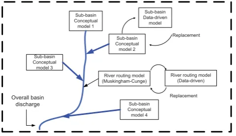
in-Sub-basin Conceptual model 1

Sub-basin Conceptual model 3

Sub-basin Conceptual

model 2

Sub-basin Conceptual

model 4

Overall basin discharge

Sub-basin Data-driven

model

Replacement

River routing model (Muskingham-Cunge)

River routing model (Data-driven)

Replacement

Fig. 1. Replacement of sub-basin models by ANN models.

volving ANN submodels, and performed additional analysis of the variations of the models seasonal performance (Fig. 1). The objectives of this paper are: (i) to analyse the per-formance of DDMs in their role as sub-basin replacements for overall flow simulations; (ii) to explore the use of an ANN routing model for the integration of sub-basin models; (iii) draw conclusions about the applicability of the hybrid process-based and data-driven models in operational flow forecasting.

2 HBV-M model for Meuse river basin

The conceptual hydrological model HBV was developed in the early 1970s (Bergstr¨om and Forsman, 1973) and its ver-sions have been applied to many catchments around the world (Lindstr¨om et al., 1997). HBV describes the most important runoff generating processes with simple and ro-bust procedures. In the snow routine, snow accumulation and melt are determined using a degree temperature-index method. The soil routine divides the forcing by rainfall and meltwater, into runoff generation and soil storage for later evaporation. The runoff generation routine consists of one upper non-linear reservoir representing fast and intermediate runoff components, and one lower linear reservoir represent-ing base flow. Runoff routrepresent-ing processes are simulated usrepresent-ing a simplified Muskingum approach and/or a triangular equi-lateral transfer function (Ponce et al., 1996).

HBV is a semi-distributed model and the river basin can be subdivided into sub-basins (HBV-S). This model simu-lates the rainfall-runoff processes for each sub-basin sepa-rately with a daily or hourly time step. Each sub-basin is divided into homogenous elevations which are then divided into vegetation zones. Further details about the HBV model can be found in Lindstr¨om et al. (1997) and Fogelberg et al. (2004).

outlets of the basins is significant. The Eq. (1) was used in this study.

Qn+1=C0In+1+C1In+C2Qn (1)

C0=

_K

x−0.51t K−Kx+0.51t

(2)

C1=

_K

x+0.51t K−Kx+0.51t

(3)

C2=

_K−K

x−0.51t K−Kx+0.51t

(4) where,Kis a storage factor with units of time, and1tis the time interval considered in the simulation. The value ofx

represents the position on the river channel in meters.Inand In+1are the inputs to the channel at the beginning and the end of the period1t, respectively.

Diermansen (2001) presented an analysis of spatial het-erogeneity in the runoff response of large and small river basins, and an increase of error is observed with an increase of the number of spatial details in the model. An alterna-tive to fully-distributed models is the class of intermediate models, the so-called semi-distributed conceptual models, as the most appropriate modelling approach for meso-scale operational forecasting. In this research the IHMS-HBV model (Lindstr¨om et al., 1997) belonging to this class is used (http://www.smhi.se). In this paper it will be called simply HBV, and will refer to the initial hydrological model formu-lation used as a hydrological prototype module in the flood early warning system for the rivers Rhine and Meuse.

Ashagrie et al. (2006) presented a long term analysis for the effects of climate change and land use change on the Meuse river basin using the HBV model. This analysis showed that the agreement between the observed and mea-sured discharge is generally good, in particular flood volumes and the highest peak are simulated well. However, there are some problems with the medium flow (shape and peak val-ues), and a systematic deviation for certain observed periods (i.e. 1930–1960) was also observed. de Wit et al. (2007b) explored the impact of climate change on low-flows. They found high accuracy for the monthly average discharge and for the highest (January) and lowest discharge (August), but there was an overestimation and underestimation observed in spring and autumn, respectively. To improve the model per-formance, various calibration techniques have been tried, e.g. Booij (2005) presented the manual calibration and validation of the HBV based on expert tuning of model parameters. The problems mentioned above still remain unresolved and under investigation by a number of authors.

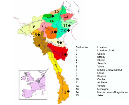
Fig. 2. The Meuse River basin and the sub-basins divisions

up-stream of Borgharen. The arrows represent the regions for which HBV-S model were replaced by ANNs (Scheme 2).

2.1 Characterisation of the Meuse River basin

The Meuse River originates in France, flows through Bel-gium and The Netherlands, and finally drains into the North Sea (Fig. 2). The river basin has an area of about 33 000 km2 and covers parts of France, Luxembourg, Belgium, Germany and The Netherlands. The length of the river from its source in France to the North Sea at the Hollands Diep (an estuary of the Rhine and Meuse rivers) is about 900 km. Major trib-utaries of the Meuse are the Chiers, Semois, Lesse, Sambre, Ourthe, Ambl`eve, Vesdre and Roer. The hydrological model of the Meuse basin upstream of Borgharen is subdivided into 15 sub-basins, covering an area of 21 000 km2(Fig. 2). For more detailed information about catchment geological and hydrological properties see Berger (1992) and de Wit et al. (2007a).

In general terms the land use in the basin is made up of 34% arable land, 20% pasture, 35% forest and 9% built up areas. Tu et al. (2004) found the coverage of forest and agri-cultural land relatively stable over the last ten years, but the forest type and management practices have changed signif-icantly. In addition to this it seems that intensification and upscaling of agricultural practices and urbanization are the most important land changes in the last century.

As far as the hydrologic properties are concerned the Meuse can roughly be split into three parts (Berger, 1992):

bed is wide. Because of that the discharge up to the mouth of the Chiers has a comparatively calm course. 2. The central reaches of the Meuse (Meuse Ardennaise),

leading from the Chiers to the Dutch border near Ei-jsden. In that section the main tributaries are Viroin, Semois, Lesse, Sambre and Ourthe. Here the Meuse transects rocky stone, resulting in a narrow river and a great slope. The poor permeability of the catchment and the steep slope of the Meuse and most of the tributaries contribute to a fast discharge of the precipitation. The contribution of the area to flood waves is great, the con-tribution to low flows is small.

3. The lower reaches of the Meuse, corresponding to the Dutch section of the river. The lower reaches them-selves may again be split into the stretches from Eijs-den to Maasbracht and from Maasbracht to the mouth. In the former part the slope is still relatively high. For the greater part the river has no weirs here. In the sec-tion the Meuse has no dikes. For those reasons the stretch above Maasbracht is occasionally reckoned as part of the Meuse Ardennaise, which in that case flows from Sedan to Maasbracht. It may be remarked that the stretch that forms the border with Belgium is called the Grensmaas (Border Meuse) in the Netherlands, and Gemeenschappelijke Maas (Common Meuse) in Flan-ders.

2.2 Data validation

The validation of the data sets presented in this paper are based on the results obtained from different researches (Booij, 2002; van Deursen, 2004; Leander and Buishand, 2007; Ashagrie et al., 2006; de Wit et al., 2007b). The model used for this study (IHMS-HBV-96) was calibrated and validated by van Deursen (2004) for the basin upstream of Borgharen over the period 1969–1984 and 1985–1998, re-spectively. The overall model error obtained in the validation was±5%. Ashagrie et al. (2006) concluded that the aver-age correlation of the HBV predictions and measured data is around 0.9, and the Nash-Sutcliffe efficiency is 0.93.

Hereafter HBV-M (HBV-Meuse) refers to the instantia-tion of the HBV rainfall-runoff model for the whole of the Meuse basin. The calibration and validation data sets used in HBV modelling were constructed in such a way that the ob-served and simulated discharges in both data sets in terms of flow volumes, and the number of flood peaks and the overall shape of the hydrographs are similar. However, initially no specific low-flow indices are used neither for calibration nor validation. Therefore in this study the results of the hydro-logical simulation of the Meuse discharges done by de Wit et al. (2007b) are used. In their study, the model was specif-ically validated against low-flow indices derived for the pe-riod 1968–1998.

The HBV-M model simulates the rainfall-runoff processes for each sub-basin separately. The sub-basins are intercon-nected within the model schematization and HBV-M simu-lates the discharge at the outfall. The schematisation and pa-rameter optimization is derived from the approach proposed by van Deursen (2004).

The Meuse basin model has been calibrated and validated using daily temperature (T) and precipitation (P) for 17 loca-tions interpolated from measurement staloca-tions, the calculated potential evapotranspiration (Epot) per subbasin, and the dis-charge (Q) at Borgharen. The interpolation of the different locations was performed using kriging (Stein, 1999).

HBV-M has been run on a daily basis using daily tem-perature, precipitation, potential evapotranspiration and dis-charge data for the period 1968–1984 (calibration) and 1985– 1998 (validation) by Booij (2002, 2005) and fine-tuned (with more detailed data) by van Deursen (2004).

Complementary information on data validation can be found in the research done by de Wit et al. (2007a). Their work presents the complete and detailed description of the hydrological data used for the model development.

3 Methodology

In this study two hybrid modelling schemes were tested. In the first one, some of the HBV-S (sub-basin) models were replaced by data-driven model representations. The sec-ond scheme is based on the replacement of the Muskingum-Cunge flow routing model (1) by an ANN model integrating the outputs of the sub-basin models.

3.1 HBV-M model setup

The model results in this study have been evaluated against the observed discharge records using (a) the volume errors (mm/yr), (b) the coefficient of efficiency (CoE) for the gaug-ing stations along the Meuse and the outlets of sub-basins and the root mean squared error (RMSE, Eq. 5); (c) the nor-malised RMSE (NRMSE, Eq. 6) (for comparing the sub-basin models with considerably different flows).

RMSE= s

Pn

i=1(Qis−Qio)2

n (5)

NRMSE= s

Pn

i=1(Qis−Qio)2 Pn

i=1(Qio−Qo)2

(6)

CoE=1−

√

SSE s

n P

t=1

(Qobs,t− ¯Qobs,t)2

whereQsis simulated discharge (m3/s);Qois observed dis-charge (m3/s); n is the number of observations, and is av-erage observed discharge (m3/s) over the whole period (all summations are run from timei=1 ton).

3.2 Scheme 1: sub-basin model replacement 3.2.1 HBV-S sub-basin models

The objective of the further analysis is to determine the av-erage error contributions of the different sub-basin models (referred to as HBV-S) to the total error of HBV-M, and hence to identify the candidate sub-basin models that would need improvement or replacement. In this modelling exer-cise the river basin behaviour during different seasons and flow regimes will be also taken into account.

3.2.2 Sub-basin error contribution

The relative error contribution from a particular HBV-S (sub-basin) model is calculated as follows. First, the HBV-M model is run and its RMSE at the outlet is calculated. Then, according to a given replacement scenario a number of input measured discharges are fed into the HBV-M. These mea-sured discharges were available only for some basins, and are the ones used for the different HBV-S model replacements scenarios. The HBV-M model is run once for each scenario. The resulting RMSE for each scenario is compared to the RMSE of the standard HBV-M. This gives the possibility of identifying the overall error variation due to the sub-basin model simulation. Such an error contribution is calculated for the different flow conditions (e.g., dry and wet seasons).

The replacement of the sub-basin models is performed in sequence: it starts with the Lorraine Sud in the direction downstream towards Borgharen, then one more sub-basin model is replaced, then yet another one, until all selected sub-models are replaced (ending at Borgharen). It is important to stress that the independent replacements of sub-basins will not allow for seeing the accumulative error reduction, which is necessary to have an overall idea of the total error of the sub-basin replacement. Two important assumption are made to be able to visualize the error contribution. First, is that the compensation of errors when adding the basin is minimal in comparison to the error of the basin contribution. The second assumption is based on the additive linear error propagation along the river basin.

3.2.3 Data-driven sub-basin models

After the error contribution of the HBV-S models are iden-tified, data-driven models (DDM) can be built for each of the sub-basins under consideration. Various data-driven tech-niques are compared to select the representative and accurate DDM. Their performances were compared to that of the ex-isting HBV-M model. Apart from that, an attempt was made to recalibrate a number of local HBV models; however, the

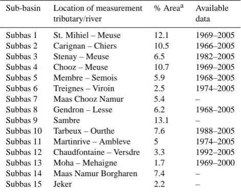
Table 1. Data available for the Meuse tributaries (catchment area

until Borgharen).

Sub-basin Location of measurement % Areaa Available

tributary/river data

Subbas 1 St. Mihiel – Meuse 12.1 1969–2005

Subbas 2 Carignan – Chiers 10.5 1966–2005

Subbas 3 Stenay – Meuse 6.5 1982–2005

Subbas 4 Chooz – Meuse 10.7 1969–2005

Subbas 5 Membre – Semois 5.9 1968–2005

Subbas 6 Treignes – Viroin 2.5 1974–2005

Subbas 7 Maas Chooz Namur 5.4 –

Subbas 8 Gendron – Lesse 6.2 1968–2005

Subbas 9 Sambre 13.1 –

Subbas 10 Tarbeux – Ourthe 7.6 1988–2005

Subbas 11 Martinrive – Ambleve 5 1974–2005

Subbas 12 Chaudfontaine – Versdre 3.3 1992–2005

Subbas 13 Moha – Mehaigne 1.7 1969–2000

Subbas 14 Maas Namur Borgharen 7.4 –

Subbas 15 Jeker 2.2 –

a_{Catchment area until Borgharen.}

overall performance obtained was lower than that after the calibration of HBV-M as a whole, and these experiments are not presented here. A detailed reference of the algorithms used can be found in Haykin (1999) and Witten and Frank (2000).

In the case study, before identifying the relative error con-tribution of various sub-basin models, several types of the DDMs were compared for 8 of 15 sub-basins. This made it possible to judge if DDMs are useful as HBV-S replace-ments.

Each data-driven rainfall-runoff model for the sub-basins uses precipitation and measured discharge as inputs, and the response discharge of the basin is generated for the moment

T time steps ahead. The general DDM forecast formulation can be represented as follows:

Qt+T =f (Rt, Rt−1, Rt−2...Rt−L, Qt...Qt−M) (8)

where the optimal lagsL for precipitation and M for dis-charge are obtained through model optimization (these can be different for various forecast horizonsT, in our case AMI and correlation results are used);f is the data-driven regres-sion model, andT is the forecast horizon (e.g. 1 day). In this research several data-driven models are tested; including linear regression model (LR, Kachroo and Liang, 1992), ar-tificial neural networks (ANN, Dawson et al., 2005 and M5 model trees (MT, Solomatine and Dulal, 2003).

have been optimized using a cross-validation set for deter-mining the number of hidden nodes.

Building M5 model trees (piece-wise linear regression models) followed the procedure presented by Witten and Frank (2000). The size of the trees is controlled by fixing of the minimum number of instances in linear regression mod-els at leaves (e.g. four).

3.3 Scheme 2: integration of sub-basin models

Routing is a common way to integrate sub-basin models of a meso-scale catchment. However, river routing models in-clude hydrodynamic conditions that require a large number of physical measurements. The accuracy is determined by the availability and the quality of these measurements and of the models. Since the cost of the measurements is high, often simplified routing equations are used. In HBV the sub-basin models use simple transfer functions that repre-sent the routing process. The main idea of the Scheme 2 is the replacement of the traditional runoff routing equations by a more accurate non-linear function (data-driven model, Fig. 3). In this paper we have chosen for the multi-layer per-ceptron ANN (ANN-MLP) due to its widely known robust-ness and accuracy. The output discharges from the fifteen HBV-S sub-basin models are lagged and used as input to this model. The lags are determined using the correlation and average mutual information analysis involving different sub-basin flows and the final outflow at Borgharen. The general ANN-MLP model to determine the flow downstream can be formulated as function of the different lags of the sub-basins.

QBorgharen_t+T =f

Q1 t−l1₁, Q

1

t−l1₂, ..., Q 1 t−l_M1 , Q

2 t−l₁2, ...,

Q2

t−l2_M, ..., Q N t−l_MN

(9) where the lower-indexT represents forecast horizon, N is the total number of sub-basins, andlk_i the lagiat each sub-basink.Mis the total number of lags taken per sub-basink. All basins in the model are lagged with respect to the current flow at Borgharen.

4 Application of Scheme 1: data-driven models for sub-basin representation

4.1 Inputs selection and data preparation for DDMs Each data set is split into a training set (70%; some data is used for cross-validation as well) and a verification (30%) set. This procedure is performed in a way that ensures that the training data contains the maximum and minimum values of each variable to reduce the possible extrapolation prob-lems. Additionally, the statistical similarity of each set was verified by comparing its probability density function. The first step in developing data-driven models for the Meuse sub-basins was to identify the most appropriate inputs for

predicting future discharges. Two approaches were used to select the appropriate input variables and their lags: correla-tion analysis and the average mutual informacorrela-tion (AMI), as it was done, for example, by Solomatine and Dulal (2003). A lag is defined as the number of time steps by which a time series is shifted relative to itself (when autocorrelated), or rel-ative to the corresponding time values of another time series (when cross-correlated). The correlation coefficient and AMI were calculated for 10 lag values. The variables compared were discharge, precipitation and evapotranspiration. Since the correlation analysis reflects only linear relationships and the phenomena are highly non-linear, the analysis based on AMI was employed as well. The AMI between two mea-surementsxi andyj drawn from setsXandY is defined by:

IXY = X

xi

yj

P(Xi,Yj)log2

_{PXY(xi, yj)}

PX(xi)PY(yj)

(10)

P(Xi,Yj)=

Z Z

XY

f (x, y)dxdy (11)

whereP(X_i,Yj) is the joint probability density for

measure-mentsXandY resulting in valuesxandy, which are the in-dividual probability density functions for the measurements ofXandY. If the measurements of a value fromX result-ing inxi is completely independent of the measurement of

a value fromY resulting inyj then the average mutual

in-formation IXY is zero. The probabilities were calculated

with different bin sizes and the results were similar. Fig-ure 4a shows the AMI for the Ourthe (a) and Lorraine Sud (b), which represent the sub-basins with faster and slower precipitation-discharge response, respectively. The maxi-mum AMI of precipitation-discharge time lag for the Ourthe corresponds to a three-day lag (Pt−3), and for the Lorraine Sud sub-basin up to a four-day lag (Pt−4)).

Based on a similar analysis to the one presented in the Fig. 4, the following model structure was adopted for eight basins:

Fig. 3. Diagram of the ANN as replacement for the routing model (Chen and Adams, 2006).

0 1 2 3 4 5 6 7 8 9 10

0.1 0.2 0.3 0.4 0.5

Correlation

Time Lag

Correlation and Average Mutual Information

0 1 2 3 4 5 6 7 8 9 100.02

0.04 0.06 0.08 0.1

AMI

Correlation AMI

0 1 2 3 4 5 6 7 8 9 10

0 0.2 0.4 0.6

Correlation

Time Lag

Correlation and Average Mutual Information

0 1 2 3 4 5 6 7 8 9 100

0.02 0.04 0.06

AMI

Correlation AMI

(a) Ourthe (b) Lorrained sud

Fig. 4. Average mutual information for between lagged precipitation and discharge for sub-basins Ourthe (a) and Lorraine Sud (b).

4.2 Data-driven sub-basin models

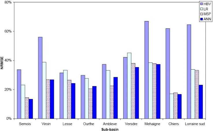
The performance of the HBV-S models was compared with that of several data-driven models (LR, M5P, ANN, Fig. 5); NRMSE was used as the error measure.

Both ANN and M5P data-driven models outperform the HBV-S models. Only for the Lesse, Ourthe, Ambleve, and Vesdre HBV-S model error is relatively low, but even then it is not comparable with that of the data-driven models. Ac-cording to Berger (1992), Ourthe sub-basin together with

Vesdre and Ambleve are the most important tributaries for flood forecasting, relating area percentage and response time. HBV-M results for Semois, Viroin, and Mehaigne show high NRMSE. The error graphs show that the M5P and ANN models outperform the HBV model for all the considered sub-basins.

Fig. 5. Comparison of model performance for each sub-basin, expressed in NRMSE of streamflow (Calculated for verification period).

discharge coming from real-time measurements preceding the forecast instant, and the conceptual model assumes that only forcing (typically precipitation and temperature) input is sufficient to drive the evolution of the system. The concep-tual model aims to represent the processes of the modelled phenomena (albeit roughly), and the DDM is based on the analysis of historical data.

Since the conceptual model only uses the forcing informa-tion (precipitainforma-tion, temperature, etc.), to obtain forecast with extended lead times in the conceptual model weather forecast information can be effectively fed into conceptual models to make forecast for longer lead times.

To obtain more accurate real-time forecasts it is often pos-sible to use the up-to-date observed system outputs in order to minimize the acknowledged errors due to the model in-adequacies (Kachroo, 1992; Moore, 1983; Schreider et al., 1997). Comparison of various updating schemes, using both types of models can be found, for example, in Toth and Brath (2007); Brath et al. (2002). Updating schemes were not con-sidered in this study but it is planned to do so.

The ANN-MLP model outperforms HBV in more cases than M5P does, and therefore is selected for the replacement experiments. The results show that DDMs can serve as ac-curate replacement models for sub-basins. However, when more and more sub-basin models are replaced, there will be less and less hydrological knowledge (encapsulated in pro-cess models) left. Therefore analysis of the overall perfor-mance of the model under different replacements has been undertaken and presented below. Since there is a large num-ber of possible scenarios of replacing various numnum-bers of models, it is necessary to analyze the river basin behaviour

and the relative quality of the individual HBV-S sub-basin models with respect to the overall basin measurements given by the discharge at Borgharen.

4.3 Analysis of HBV-S simulation errors

The changes in the overall model performance (RMSE) on the verification data set as a result of various replacements with measured discharge data are shown in Fig. 6 and Ta-ble 2.

The replacement order can be followed by reading Fig. 6 from top to bottom. From the total RMSE of 83.84, Chiers has the largest relative error contribution of 4.53% (10.5% of the total area), followed by Lorraine Sud (2) and Lesse sub-basins with an error contribution of 3.86% (12.10% of the total area) and 2.81%, respectively. Chiers is the sec-ond largest sub-basin of the Meuse and it is known that it commonly influences floods generated by its slow response, Lorraine Sud is also a slow responding basin. Vesdre, Am-bleve, Viroin and Ourthe basins closer to the outlet are the most accurate in the HBV-M model and are the ones directly responsible for floods.

Table 2. RMSE error contribution to the HBV overall simulation.

Sub-basin Relative error reduction Area Area Observed – Simulated HBV-M (RMSE, m3/s) (km2) (% of total basin) (% Volume Difference)

Mehaigne 0.87 346 1.65 1.04

Ambleve 1.44 1050 5.00 1.72

Ourthe 1.89 1597 7.60 2.26

Lesse 2.36 1311 6.24 2.81

Viroin 1.08 526 2.50 1.29

Semois 1.35 1235 5.88 1.61

Chiers 3.79 2207 10.51 4.53

Lorraine Sud 3.23 2540 12.10 3.86 Others 67.82 10 188 48.51 80.89 Total HBV error 83.84 21 000 100 100

Fig. 6. Percentage of sub-basin models errors for dry and wet seasons.

Since it is well known that seasonality influences this river basin, the error contributions of the HBV-S models in sum-mer (May–October) and winter (November–April) seasons are calculated in terms of the percentage of error with re-spect to the total HBV-M error; see Fig. 6. The results in Fig. 6 show that there is a homogeneous error contribution from Chiers in both seasons. The model for Lorraine Sud basin has a higher error contribution for summer and a small overall contribution in the winter. Clearly the calibration of the model is well suited for summer conditions where the slow response of the catchment is important for the average discharge in these periods. This is congruent with the size (2540 km2), which represents approximately 10% of the con-sidered area.

In terms of flood forecasting at Borgharen the most sen-sitive basins for the HBV-M model distribution are Ourthe, Vesdre and Ambleve. The analysis shows that the Ourthe and Ambleve stream flows do not influence the model in the summer period, but together make a significant contribution to the error generated in the winter season. The contributions

of the Mehaigne and Viroin sub-basins do not depend on the season: they have a small and similar error percentage for both seasons.

4.4 Replacements of sub-basin models by ANNs There are numerous replacement scenarios and these should be identified based not only on the previous error analysis, but also taking into account the river basin behaviour during the different seasons and the different flow regimes. The total number of possible replacement scenarios (combinations of the sub-basin models with the data availability) is too high and it is not feasible to analyze them all. The experiments to replace a sub-basin model were carried out using only 8 scenarios as shown in Table 3.

Table 3. Replacement scenarios and the effect of their implementation.

Short Replacement PARa ADCb RMSE RMSE ANN_MD−S (%) Name (%) (%) Reduction (ANN-S) ReductioncMD

R1 Chiers 11 10 3.84 4.53 0.85

R2 Chiers, Semois, Viroin 19 22 6.17 7.42 0.83 R3 Ourthe and Ambleve 13 15 2.25 3.98 0.57 R4 Ourthe, Ambleve, Lesse 19 21 4.21 6.79 0.62 R5 Ourthe Ambleve, Semois 18 25 3.73 5.58 0.67 R6 Semois, Chiers, Lesse 24 28 7.52 8.39 0.9 R7 Ourthe, Ambleve, Semois, Lesse, Chiers 35 41 8.62 12.92 0.67 R8 Lorraine Sud, Chiers, Semois 28 28 9.47 9.99 0.95

a_{Percentage of area replaced of the total basin (PAR).}

b_{Average discharge contribution in relation to the total average discharge (ADC). The total average discharge is calculated using the average}

annual discharge from 1970 to 2000 (280.1 m3/s).

c_{Measured data (MD).}

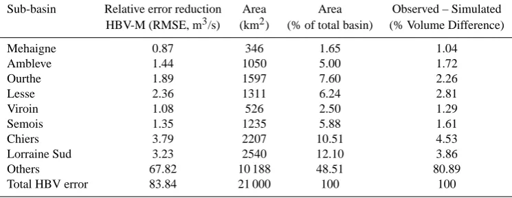
(a) Sub-basin 1 (St. Mihiel – Loraine Sud) (b) Sub-basin 2 (Chiers)

(c) Sub-basin 3 (Stenay-Meuse) (d) Sub-basin 4 (Chooz-Meuse)

– R1: the sub-basin (Chiers) with the largest error contri-bution, and a slow runoff response.

– R2: three sub-basins which include the Meuse tribu-taries upstream of Chooz. These are the highest eleva-tion areas with relatively low slope and slow response during flood situations.

– R3: the two fast responding sub-basins that have high contributions during floods (Berger, 1992).

– R4: the same sub-basins as in R3, but together with the slow response Lesse sub-basin whose model has a high error in summer and a low error in winter.

– R5: the same sub-basins as in R3, but together with the slow responding Semois whose model has a high error in summer and low error in winter.

– R6: combination of slow and fast responding sub-basins.

– R7: combinations of slow and fast responding sub-basins, but with a larger area covering 35% of the basin. – R8: slow responding sub-basins with a large total area. Table 3 presents the HBV-M model performance changes as a consequence of the different ANN-S replacement strate-gies. The following statements describe the interpretation of some of the results:

The effectiveness of the models replacements can be eval-uated by analysing the changes in the overall HBV-M RMSE. The last column presents the percentages of the maximum reduction possible in case of implementing a particular re-placement scenario.

Comparing sub-basins with similar area and similar dis-charge we can see where the replacement of models was more successful. For example R1 and R3 have similar per-centage of area (11 and 13, respectively), also similar aver-age discharge contribution (10 and 15, respectively). How-ever, the R1 (ANN-S) model gives a RMSE reduction (85%), which is higher than that for the scenarios R3, corresponding to larger areas and higher average discharge. This is an in-dicator that low flows play a significant role in the overall process, and also reflects the weakness of the HBV-S models currently used in simulating low flows.

A similar situation can be observed when R7 replaced a bigger area (35%) than R8 (28%), however, the efficiency for the latter replacement is significantly higher (95%). In terms of discharge, R8 has a smaller average discharge and there-fore less contribution. For the scenarios R6 and R8 results show a similar error reduction after the replacement. They have approximately the same average discharge percentage contribution to the basin and a similar area, however, their seasonal error contribution is different (Fig. 6).

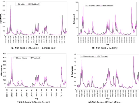
The influence of changing Ourthe and Ambleve for Lor-raine Sud shows that most of the errors arise in the low flow

Fig. 8. Hydrograph replacements (R8) and (R6).

modelling. The Lorraine Sud is the most distant basin with relatively mild slope, and therefore its contribution to flash flood (fast flow and runoff) is minimal. This is consistent with the results of de Wit et al. (2007b), who showed that the peak discharges of Vesdre and Ourthe basins are larger than those of Chooz. The results point to a partial explanation based on the differences in precipitation depths of the region and on the difference in hydro-geological conditions. On the other hand, the basins Ourthe and Ambleve (central part) are closer to the outlet and their individual performances are more sensitive for short time lags and fast phenomena.

The results of simulations for the verification period (last three years) are evaluated by calculating the RMSE and Co-efficient of efficiency (Fig. 9). A typical section of the hy-drograph is extracted in Fig. 8. The shape of the hyhy-drograph with ANN-S replacement is mainly driven by the overall hy-drological model. It is possible to see that after the replace-ment R8 the flows under 600 m3/s are closer to the observed discharge. For flows above 600 m3/s the HBV-M is hardly af-fected due to the low influence of the replaced basins during the peak flow events (Fig. 8). This shows that the replace-ment affects mainly the low flow simulation periods.

If one analyses only the reduction in the overall RMSE, then the replacement scenario R8 would result in the model that can be recommended to use instead of the HBV-M.

5 Application of Scheme 2: integrating sub-basin models by ANN

83.8

80.0

77.7 81.6

79.6 80.1

76.3

75.2

74.4

68 70 72 74 76 78 80 82 84 86

HBV-1 R1 R2 R3 R4 R5 R6 R7 R8

Model set-up

RMSE

0.85 0.86

0.87

0.86 0.86

0.86 0.87

0.88 0.88

0.830 0.840 0.850 0.860 0.870 0.880 0.890

HBV-1

R1 R2 R3 R4 R5 R6 R7 R8

Model set-up

Coefficient of Efficiency

RMSE Coefficient of efficiency

Fig. 9. Error reduction with different combinations of replacement (evaluated at Borgharen).

0 500 1000 1500 2000 2500

−500 0 500 1000 1500 2000 2500

Measured discharge (m³/s)

Simulated discharge (m³/s)

Data Points Best Linear Fit Y = T

R=0.9673

Linear fit: Y=(0.94)T+(15)

0 500 1000 1500 2000 2500 3000

−500 0 500 1000 1500 2000 2500 3000

Measured discharge (m³/s)

Simulated discharge (m³/s)

Linear fit: y = 0.98*x − 1 Data Points

linear Best Linear Fit Y = T

(a) Training (b) Verification

Fig. 10. Scatter plots of target (measured) and ANN model for training and verification period.

AMI related to the observed discharge at Borgharen is a time lag of 1 day. Exceptions are sub-basins 9 (Sambre), 10 (Our-the), 13 (Mehaigne), and 15 (Jeker) since the corresponding AMI is at maximum for lags less than 1 day. Therefore in Eq. 8, only 1 day lags is considered for all basins. Fifteen

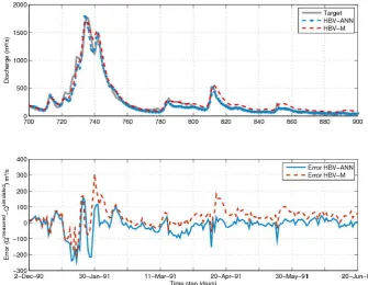
Fig. 11. Hydrograph of the original HBV-M and HBV-ANN integrated models.

a day. More precise time lags can be obtained with hourly data. The average travel time of the flow between the Semois measuring station (sub-basin 5) and Borgharen is one day (Berger, 1992).

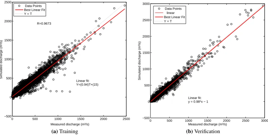
The results of the model can be visualized by scatter plots. High correlations are found between the observed and simulated discharge both for training and verification sets (Fig. 10).

Figure 11 shows the observed and simulated discharges at Borgharen from 2 December 1990 (record 700) to 20 June 1991 (record 900). On average the integrated HBV-ANN model outperforms the original HBV-M model. The reces-sion curve of the hydrograph is clearly closer to the measured curve and what was viewed as the systematic error in the re-cession curve of the HBV-M model is now corrected. An interesting phenomenon can be observed close to the mea-sured peak: the measurement value goes up and down before it reaches its maximum value. This peak change in the hy-drograph is reproduced by the ANN routing model with a relatively small underestimation.

For a 3 years error analysis the HBV-ANN gives RMSE of 58.66 m3/s. An extended error analysis of nine years ver-ification period shows that the RMSE for the HBV-M and HBV-ANN are 86 m3/s and 55 m3/s respectively which is a 36% improvement (Table 4). The coefficient of efficiency is also improved from 0.918 for the M to 0.967 for HBV-ANN model. For both winter and summer seasons it is clear that the use of ANN for integrating the sub-basin models im-proves the accuracy.

5.1 Integrating Schemes 1 and 2

The ANN-MLP routing model integrates the results of the sub-basin models and generates the value of discharge at the outlet (Borgharen). By doing so, the ANN routing is already correcting the regional behaviour of each sub-basin model, so the ANN-MLP routing acts as an error corrector. There-fore, the use of another sub-basin model (e.g. R8 scenario in Table 3), with different error performance, as input of the ANN-routing model does not add new knowledge into the model, but only increases the error. The replacement R8 into the ANN-MLP (scheme) had almost the same performance as the original HBV without any replacement (RMSE 82.91, see Fig. 12).

6 Discussion

In this section the results for each scheme are discussed and compared.

6.1 Scheme 1

Table 4. Comparison between the HBV-M model and the integrated HBV-ANN model.

Hydrological year (Nov–Oct) Winter (Nov–Apr) Summer (Apr–Oct) Model HBV-1 HBV-ANN HBV-1 HBV-ANN HBV-1 HBV-ANN RMSE (m3/s) 85.65 54.51 100.02 64.26 71.66 45.56 NRMSE 0.29 0.18 0.27 0.18 0.48 0.31

Fig. 12. Hydrograph comparison for the HBV-ANN with and without R8 replacement.

forecast, however, whereas the ANN models only previous measured discharge is needed. Therefore, this approach may bring operational advantages on the locations where weather forecast information may not be available.

The choice of the best combination of HBV and ANN components depends on various factors and is, in fact, a multi-criteria problem. One may also think of rules (taking into account for example the season, data availability, loca-tion) that decision maker would use to select the final model. The use of Scheme 1 may well be suited for simulation, but comparative tests with data-assimilation and data-driven approaches of the whole basin may be needed to determine whether the use of data-assimilation in operational system is more accurate or suitable than a simple ANN model of a basin. This analysis will be conducted in further studies.

Note that the extended forecast made by DDMs can be produced in different ways. Simply using previously simu-lated discharges in an autoregressive conceptualization might be the most straightforward approach. Another approach was explored by Toth and Brath (2007); Corzo and Solomatine (2007a), where separate ANNs were created for each lead time value.

Three important implications have to be mentioned here. Firstly, the use of previously simulated discharges iteratively decreases the quality of the forecast. Secondly, if we assume that the measured information is a perfect forecast, the HBV average performance will not decrease for higher forecast horizons. Thirdly, the DDM is not representing the basin behaviour and instead is acting more as an autoregressive model with a small component given by the precipitation.

The data-driven model, which tends to generate high weight values for input from previous discharges in its struc-ture, underestimate the use of other variables that are poorly correlated with the output. In this sense data-driven models (DDM) can simulate the flow quite accurately (only on aver-age, however, and not in the beginning of a high precipitation event) even without the use of the variables that really drive the phenomena (precipitation and temperature).

6.2 Scheme 2

routing scheme employed in the HBV-M model. Our results in this experiment are in agreement with the work by Chen and Adams (2006) where an ANN model was used to inte-grate the three basin models (Xinanjiang model, Tank model, and Soil Moisture Accounting model).

Scheme 2 does not only consider the integration of stream-flow process, but can be also seen as a data assimilation ap-proach (error corrector). Note that the ANN-MLP model does not target the accurate representation of the physical system dynamics; instead, the target is aimed to reproduce the measured value (discharge).

The use of physical conceptual and data-driven models in operation should consider the dynamics of the basin. The dy-namics of the Meuse basin has hardly changed during the last decade (Tu et al., 2004), so the combination of models seems to be reliable under relatively long periods of time (e.g. 3 to 5 years as the validation period of the models presented).

It should be noted that the experiments presented in this paper are based on daily data and are aimed at improving the HBV-M hydrological model. In subsequent studies it is planned to explore the usefulness of the approaches above under a more detailed and complex framework (daily fore-cast with hourly data and precipitation forefore-cast information). The challenge in extending these concepts to hourly-based models relates not only to the non-linearity and dynamics, but also to the influence of human interventions at weirs, sluices, canals, power plants, etc. These aspects are not in-cluded in the HBV-M model and are part of the motivation to use data-driven techniques, and, possibly, rule-based tech-niques allowing for multiple regimes of model operation.

7 Conclusions

This paper explored two schemes of introducing data-driven model components into a semi-distributed process based rainfall-runoff model. The first scheme explored the replace-ment of HBV sub-basin models by ANN-MLP models using several scenarios. The results show that such approach im-proves the discharge simulation both in terms of reducing the RMSE and increasing the model efficiency. The improve-ment was mainly observed for the summer periods for low flows.

The second scheme used the replacement of the routing model (combining the individual sub-basin models) by an ANN, and lead to higher gains in terms of the overall error than the first scheme. Nevertheless, it is important to stress that this latter scheme does not only reproduce the flow, but also the noise in the system. The use of an ANN for routing replacement is not only a simulation tool but also captures the variation in the time series. Therefore, its results can not be interpreted as the accurate representation of the river rout-ing but more as a tool to combine the model’s and which acts as an error corrector as well.

In general it can be concluded that the both combination schemes have a clear potential in improving the accuracy of the considered class of hydrological models.

Performance of operational systems is typically affected by the limited and/or inaccurate data. A possible way to al-leviate this, is to use autoregressive models which are not sensitive to the precipitation, temperature and evapotranspi-ration. Yet another issue is the estimation of the models un-certainty associated with the inaccuracies in data and model structures. It is planned to explore all these issues and possi-bilities in further studies.

Acknowledgements. Measurement data for each sub-basin of the

HBV model was collected from the “Direction g`en`erale des Voies hydrauliques Belgian” (http://voies-hydrauliques.wallonie.be) and from the Minist`ere de l’ecologie et du d`eveloppement durable (http://www.hydro.eaufrance.fr). The authors appreciate the support through the Delft Cluster research programme of the Dutch Government (project “Safety against flooding”) and of the UNESCO-IHE Institute for Water Education for supporting this research. We would also like to thank Mr. A. G. Ashagrie who provided us with some valuable data sets. Our gratitude goes also to Editor E. Toth for her useful comments helping to improve the manuscript.

Edited by: E. Toth

References

Abrahart, R. J. and See, L.: Multi-model data fusion for river flow forecasting: an evaluation of six alternative methods based on two contrasting catchments, Hydrol. Earth Syst. Sci., 6, 655–670, 2002, http://www.hydrol-earth-syst-sci.net/6/655/2002/. Anctil, F. and Tap´e, D. G.: An exploration of artificial neural

net-work rainfall-runoff forecasting combined with wavelet decom-position, J. Environ. Eng. Sci, 3(1), S121–S128, 2004.

ASCE: Task Committee on Application of Artificial Neural Net-works in Hydrology, Artificial Neural NetNet-works in Hydrology. II: Hydrologic Application, J. Hydrol. Eng., 5, 124–136, 2000. Ashagrie, A. G., de Laat, P. J., de Wit, M. J., Tu, M., and

Uhlen-brook, S.: Detecting the influence of land use changes on dis-charges and floods in the Meuse River Basin - the predictive power of a ninety-year rainfall-runoff relation?, Hydrol. Earth Syst. Sci., 10, 691–701, 2006,

http://www.hydrol-earth-syst-sci.net/10/691/2006/.

Berger, H. E. J.: Flow Forecasting for the River Meuse, Technische Universiteit Delft, 1992.

Bergstr¨om, S. and Forsman, A.: Development of a conceptual deter-ministic rainfall-runoff model, Nord. Hydrol., 4, 147–170, 1973. Booij, M. J.: Modelling the effects of spatial and temporal reso-lution of rainfall and basin model on extreme river discharge, Hydrolog. Sci. J., 47, 307–320, 2002.

Booij, M. J.: Impact of climate change on river flooding assessed with different spatial model resolutions, J. Hydrol., 303, 176– 198, 2005.

Brath, A., Montanari, A., and Toth, E.: Neural networks and non-parametric methods for improving real-time flood forecasting through conceptual hydrological models, Hydrol. Earth Syst. Sci., 6, 627–639, 2002,

http://www.hydrol-earth-syst-sci.net/6/627/2002/.

Chen, J. and Adams, B. J.: Integration of artificial neural networks with conceptual models in rainfall-runoff modeling, J. Hydrol., 318, 232–249, 2006.

Corzo, G. and Solomatine, D.: Knowledge-based modularization and global optimization of artificial neural network models in hydrological forecasting, Neural Networks, 20, 528–536, 2007a. Corzo, G. A. and Solomatine, D. P.: Baseflow separation techniques for modular artificial neural networks modelling in flow forecast-ing, Hydrolog. Sci. J., 52, 491–507, 2007b.

Dawson, C. W., See, L. M., Abrahart, R. J., Wilby, R. L., Sham-seldin, A. Y., Anctil, F., Belbachir, A. N., Bowden, G., Dandy, G., and Lauzon, N.: A comparative study of artificial neural net-work techniques for river stage forecasting, in: Proceedings of IEEE International Joint Conference on Neural Networks, Mon-treal, Que., 4, 2666–2670, 2005.

de Wit, M. J. M., Peeters, H. A., Gastaud, P. H., Dewil, P., Maeghe, K., and Baumgart, J.: Floods in the Meuse basin: event descrip-tions and an international view on ongoing measures, Interna-tional Journal of River Basin Management, 5, 279-292, 2007a. de Wit, M. J. M., van den Hurk, B., Warmerdam, P. M. M., Torfs, P.,

Roulin, E., and van Deursen, W. P. A.: Impact of climate change on low-flows in the river Meuse, 2007b.

Dibike, Y., Velickov, S., Solomatine, D., and Abbott, M.: Model Induction with Support Vector Machines: Introduction and Ap-plications, J. Comput. Civil Eng., 15, 208–216, 2001.

Dibike, Y. B. and Abbott, M. B.: Application of artificial neural networks to the simulation of a two dimensional flow, J. Hydraul. Res., 37, 435–446, 1999.

Diermansen, F.: Physically based modelling of rainfall-runoff pro-cesses, Ph.D. Thesis – TuDelft, 123–150, 2001.

Fenicia, F., Solomatine, D. P., Savenije, H. H. G., and Matgen, P.: Soft combination of local models in a multi-objective framework, Hydrol. Earth Syst. Sci., 11, 1797–1809, 2007,

http://www.hydrol-earth-syst-sci.net/11/1797/2007/.

Fogelberg, S., Arheimer, B., Venohr, M., and Behrendt, H.: HBV modeling in several European countries, Proceedings of Nordic Hydrologic conference, 2004.

Haykin, S.: Neural networks: a comprehensive foundation, Prentice Hall, second edn., 1999.

Kachroo, R.: River Flow Forecasting. Part 2. Applications of a con-ceptual model, J. Hydrol., 7(133), 141–178, 1992.

Kachroo, R. and Liang, G.: River Flow Forecasting. Part 2. Alge-braic Development of Linear Modelling Techniques, J. Hydrol., 133, 17–40, 1992.

Leander, R. and Buishand, T. A.: Resampling of regional climate model output for the simulation of extreme river flows, 2007. Levenberg, K.: A method for the solution of certain problems in

least squares, Quart. Appl. Math, 2, 164–168, 1944.

Linde, A. T., Hurkans, R., Aerts, J., and Dolman, H.: Comparing model performance of the HBV and VIC models in the Rhine basin, in: Symposium HS2004 at IUGG2007, IAHS, Perugia, 278–285, 2007.

Lindstr¨om, G., Johansson, B., Persson, M., Gardelin, M., and Bergtr¨om, S.: Development and test of the distributed HBV-96 hydrological model, J. Hydrol., 201, 272–228, 1997.

Marquardt, D.: An algorithm for least-squares estimation of nonlin-ear parameters, SIAM J. Appl. Math., 11, 431–441, 1963. Moore, R.: Flood forecasting techniques, Tech. rep., I.

WMO/UNDP Regional Training seminar on flood forecasting, Bangkok, Thailand, 1983.

NERC: Flood Studies Report, Vol. 5: Flood Routing Studies., Tech. rep., Natural Environment Research Council, London, 1975. Nilsson, P., Uvo, C. B., and Berndtsson, R.: Monthly runoff

simula-tion: Comparing and combining conceptual and neural networks models, J. Hydrol., 321, 344–363, 2006.

Ponce, V. M., Lohani, A. K., and Scheyhing, C.: Analyti-cal verification of Muskingum-Cunge routing, J. Hydrol., 174, 235–241, doi:10.1016/0022-1694(95)02765-3, http: //www.sciencedirect.com/science/article/B6V6C-3VW173F-3/ 2/842b6f3ce5b836f6b48ebf8347774b88, 1996.

Schreider, S., Jakeman, A., Dyer, B., and Francis, R.: A combined deterministic and self-adaptive stochastic algorithm for stream-flow forecasting with application to catchments of the Upper Murray Basin, Australia, Environ. Modell. Softw., 12, 93–104, 1997.

Seibert, J.: Estimation of parameter uncertainty in the HBV model, Nord. Hydrol., 28, 247–262, 1997.

Solomatine, D. P. and Dulal, K. N.: Model tree as an alternative to neural network in rainfall-runoff modelling, Hydrolog. Sci. J., 48, 399–411, 2003.

Solomatine, D. P. and Price, R. K.: Innovative approaches to flood forecasting using data driven and hybrid modelling, in: 6th In-ternational Conference on Hydroinformatics, edited by: Liong, Phoon, and Babovic, 1639–1646, World Scientific Publishing Company, Singapore, 1639–1647, 2004.

Stein, M.: Interpolation of Spatial Data: Some Theory for Kriging, Springer, 1999.

Toth, E.: Classification of hydro-meteorological conditions and multiple artificial neural networks for streamflow forecasting, Hydrol. Earth Syst. Sci. Discuss., 6, 897–919, 2009,

http://www.hydrol-earth-syst-sci-discuss.net/6/897/2009/. Toth, E. and Brath, A.: Multistep ahead streamflow

fore-casting: Role of calibration data in conceptual and neu-ral network modeling, Water Resour. Res., 43, W11405, doi:10.1029/2006WR005383, 2007.

Tu, M., Hall, M., and Laat, P. D.: Detection of long-term changes in precipitation and discharge in the Meuse, GIS and remote sens-ing in Hydrology, Water resources and enviromental – Proceed-ings of the international conference of the ICGRHWE held at the Three Gorges Dam, China, Septembre 2003, IAHS Publ. 289, 2004.

van Deursen, W.: Calibration HBV model Meuse, Tech. rep., Carthago Consultancy, 2004.