Hydrol. Earth Syst. Sci., 17, 445–452, 2013 www.hydrol-earth-syst-sci.net/17/445/2013/ doi:10.5194/hess-17-445-2013
© Author(s) 2013. CC Attribution 3.0 License.
EGU Journal Logos (RGB)
Advances in
Geosciences
Open Access
Natural Hazards
and Earth System
Sciences
Open AccessAnnales
Geophysicae
Open AccessNonlinear Processes
in Geophysics
Open AccessAtmospheric
Chemistry
and Physics
Open AccessAtmospheric
Chemistry
and Physics
Open Access DiscussionsAtmospheric
Measurement
Techniques
Open AccessAtmospheric
Measurement
Techniques
Open Access DiscussionsBiogeosciences
Open Access Open Access
Biogeosciences
Discussions
Climate
of the Past
Open Access Open Access
Climate
of the Past
Discussions
Earth System
Dynamics
Open Access Open Access
Earth System
Dynamics
DiscussionsGeoscientific
Instrumentation
Methods and
Data Systems
Open Access
Geoscientific
Instrumentation
Methods and
Data Systems
Open Access DiscussionsGeoscientific
Model Development
Open Access Open Access
Geoscientific
Model Development
DiscussionsHydrology and
Earth System
Sciences
Open AccessHydrology and
Earth System
Sciences
Open Access DiscussionsOcean Science
Open Access Open Access
Ocean Science
Discussions
Solid Earth
Open Access Open Access
Solid Earth
Discussions
The Cryosphere
Open Access Open Access
The Cryosphere
DiscussionsNatural Hazards
and Earth System
Sciences
Open Access
Discussions
An educational model for ensemble streamflow simulation
and uncertainty analysis
A. AghaKouchak1, N. Nakhjiri1, and E. Habib2 1University of California Irvine, Irvine, CA 92697, USA
2University of Louisiana at Lafayette, Lafayette, Louisiana, 70504, USA
Correspondence to: A. AghaKouchak ([email protected])
Received: 17 May 2012 – Published in Hydrol. Earth Syst. Sci. Discuss.: 8 June 2012 Revised: 16 January 2013 – Accepted: 16 January 2013 – Published: 1 February 2013
Abstract. This paper presents the hands-on modeling tool-box, HBV-Ensemble, designed as a complement to theoret-ical hydrology lectures, to teach hydrologtheoret-ical processes and their uncertainties. The HBV-Ensemble can be used for in-class lab practices and homework assignments, and assess-ment of students’ understanding of hydrological processes. Using this modeling toolbox, students can gain more in-sights into how hydrological processes (e.g., precipitation, snowmelt and snow accumulation, soil moisture, evapotran-spiration and runoff generation) are interconnected. The ed-ucational toolbox includes a MATLAB Graphical User Inter-face (GUI) and an ensemble simulation scheme that can be used for teaching uncertainty analysis, parameter estimation, ensemble simulation and model sensitivity. HBV-Ensemble was administered in a class for both in-class instruction and a final project, and students submitted their feedback about the toolbox. The results indicate that this educational soft-ware had a positive impact on students understanding and knowledge of uncertainty in hydrological modeling.
1 Introduction
Rainfall–runoff models have been used to describe nonlinear hydrological processes, predict extreme events and assess the impacts of potential changes in future climates and/or land use. Numerous physical, conceptual, and statistical models have been used for modeling rainfall–runoff processes (e.g., Singh and Woolhiser, 2002; Beven, 2001; Bergstr¨om, 1995; Wheater et al., 1993). Given the importance of water re-sources and the significance of hydrologic extremes on hu-man livelihood and society, educating students on various
aspects of the hydrological cycle is very important. However, reliable rainfall–runoff modeling and flood management en-tails a strong background in the hydrological cycle and mod-eling, which students may not have.
The United States National Research Council has also stressed the need for an improve hydrology curriculum, specifically in the areas of hydrologic modeling and data analysis (e.g., NRC, 2000, 1991; Wagener et al., 2012). In a report by the Consortium for Universities for the Ad-vancement of Hydrologic Science (CUAHSI), the potential role of hydrologic models in transforming the way hydrol-ogy is taught and communicated to students is emphasized (CUAHSI, 2007).
Recent research on engineering and science education sug-gests that students acquire a better knowledge of hydrologi-cal processes and their uncertainties when exposed to novel educational techniques (e.g., student centered methods) as a complement to traditional lecture-driven classes (see Thomp-son et al., 2012 and references therein). Wagener et al. (2010) argue that the changing demands on hydrology offers an unprecedented opportunity to advance hydrology education. Recent advances in simulation models, graphical user inter-face developments and physical models provide opportuni-ties for improving existing hydrology curriculum (see Shaw and Walter, 2012; Habib et al., 2012; Pathirana et al., 2012; Seibert and Vis, 2012a; Rusca et al., 2012; Rodhe, 2012; AghaKouchak and Habib, 2010).
In a recent study, AghaKouchak and Habib (2010) intro-duced HBV-EDU which is a hands-on modeling tool devel-oped for students to help them learn the fundamentals of hy-drological processes, parameter estimation and model cali-bration. HBV-EDU provides an application-oriented learn-ing environment that introduces the interconnected hydro-logical processes through the use of a simplified concep-tual hydrologic model. Using HBV-EDU, students can prac-tice conceptual thinking in solving hydrology problems. Using a detailed course survey, AghaKouchak and Habib (2010) showed that students were more inspired by hands-on applicatihands-on-oriented teaching methods (e.g., using mod-els) than by purely theoretical lecture driven classes. Seibert and Vis (2012b) presented HBV-light which is also a user-friendly conceptual model, especially useful for teaching hy-drological modeling and uncertainty estimation. The model includes different functionalities such as automatic calibra-tion and Monte Carlo simulacalibra-tions designed for teaching ad-vanced hydrology classes and research projects.
Like HBV-EDU, most hydrologic models used for both teaching and research are deterministic, providing the best simulation based on estimated parameters (e.g., Beven, 2001; Young, 2002). However, quantification of uncertainties asso-ciated with hydrologic models are fundamental for risk as-sessment and decision making. To accomplish this, ensemble streamflow simulation can be used for uncertainty analysis, risk assessment and probabilistic analysis of flood forecasts (Beven, 2008; Wood et al., 2002; Georgakakos et al., 2004; Vrugt et al., 2008). For example, using ensemble stream-flow simulations, one can derive the probability of the wa-ter level exceeding a certain extreme threshold. Also, the ef-fect of the uncertainty in observations, model representations of hydrological processes, and global climate studies has been highlighted in numerous studies (Bell and Moore, 2000; Goodrich et al., 1995; AghaKouchak et al., 2010; Obled et al., 1994; AghaKouchak et al., 2012).
The concepts of ensemble simulation and uncertainty anal-ysis are typically covered in hydrology classes only theoreti-cally. Several models and tools have been used for estimation of uncertainty of hydrologic models and for teaching pur-poses (e.g., Rainfall–Runoff Modelling Toolbox – RRMT, Wagener et al., 2004; HBV-light; Seibert and Vis, 2012b; GLUE Software, GLUEWIN; Beven and Binley, 1992). We hypothesize that the students would gain a better knowl-edge of model uncertainty using educational simulation tools and techniques. There are different approaches to uncertainty estimation including statistical methods, and physical and non-statistical methods (see Beven and Kimberlain, 2009; Montanari et al., 2009). This study builds upon the previous model (HBV-EDU) and provides an educational software for teaching ensemble simulation and uncertainty analysis using a statistical approach. The modeling toolbox, named HBV-Ensemble, provides an ensemble of streamflow simulations based on randomly selected parameters that satisfy a cer-tain objective function. The aim of HBV-Ensemble is both
to teach both hydrological processes and uncertainty estima-tion. HBV-Ensemble can be employed for in-class lab prac-tices and assignments as well as assessment of students’ un-derstanding of hydrological processes. We anticipate that the presented educational toolbox to encourage students to learn more about the fundamentals of hydrology, ensemble simu-lation and uncertainty analysis. Notice that an ensemble is often described as simulations from different models. In this paper, an ensemble is defined as multiple simulations using different sets of parameters (e.g., Beven and Freer, 2001; Re-nard et al., 2010; Wagener, 2003; Murphy et al., 2004; Piani et al., 2005).
The paper is organized into five sections. After this intro-duction, the model concept and methodology are briefly in-troduced. In the third section, an example application of the toolbox is presented. The fourth section is devoted to the stu-dents feedback. Finally, the last section summarizes the re-sults and conclusions.
2 Methodology and model concept
2.1 HBV model
The proposed model is based on the a modified version of HBV hydrologic model (Bergstr¨om, 1995). The model is originally developed by the Swedish Meteorological and Hy-drological Institute. Various versions of the model are now available that vary in complexity and utility features. The hydrological model used in HBV-Ensemble is a modified version of the HBV presented in Hundecha and B´ardossy (2004) and AghaKouchak and Habib (2010). The HBV-Ensemble consists of five main modules: (1) snowmelt and snow accumulation; (2) soil moisture and effective precipita-tion; (3) evapotranspiraprecipita-tion; (4) runoff response; (5) ensem-ble simulation. A detailed discussion on the HBV model is provided in this Special Issue (see Seibert and Vis, 2012b) as well as in Hundecha and B´ardossy (2004) and AghaKouchak and Habib (2010). For this reason, only a brief overview of the model is presented here.
In this model, observed precipitation partitions into rain-fall and snow based on observed temperature. As long as the temperature remains below the melting threshold snow ac-cumulates, and for temperatures above the melting thresh-old snow melts (see Seibert and Vis, 2012b for the gov-erning equations). This approach is known as the degree-day method. The combination of rainfall and snowmelt will then be partitioned into direct (surface) runoff and infiltration based on the soil moisture condition.
the near surface flow and the lower reservoir simulates the base flow (groundwater flow). A constant percolation rate is used to connect the reservoirs. The upper reservoir has two outlets for estimation of the near surface flow and interflow, whereas the lower reservoir has one outlet for simulation of the baseflow. The total surface water (runoff) would then be derived as the sum of the outflows from both reservoirs.
2.2 Ensemble simulation module
HBV-Ensemble provides an educational software for teach-ing ensemble simulation and uncertainty analysis. In HBV-Ensemble a range of model parameters are sampled using the Monte Carlo technique and all simulations that satisfy the ob-jective function will be accepted as one realization in the en-semble output. A common objective function is the Nash— Sutcliffe coefficient (Nash and Sutcliffe, 1970):
RNS=1−
6tn=1 Qts−Qto2
6nt=1 Qt o−Qo
2, (1)
whereRNS= Nash–Sutcliffe coefficient [−];Qs= simulated discharge [L3T−1]; Qo= observed discharge [L3T−1]; Oo= mean observed discharge [L3T−1]; andn= number of time steps. The model parameters of HBV-Ensemble include: degree-day factor; field capacity; shape coefficient; evapo-transpiration adjustment parameter; permanent wilting point; near surface flow, interflow and baseflow constants; percola-tion storage constant; and threshold water level for near sur-face flow. For a detailed discussion on the parameters, the reader is referred to Seibert and Vis (2012b) and AghaK-ouchak and Habib (2010). The procedure to generate an en-semble of streamflow simulations is as follows:
1. Select reasonable upper and lower bounds for the model parameters mentioned above based on expert knowl-edge, available data or literature.
2. Draw random samples of parameters from the above range (e.g., 1000 sets of randomly selected parame-ters) using the Generalized Likelihood Uncertainty Es-timation (GLUE; Beven and Binley, 1992 – see GLUE demonstration software available through the Lancaster University for more information).
3. Run HBV-Ensemble with all parameter combinations obtained from the previous time step.
4. Accept simulations (ensemble members) and parameter sets that satisfy a certain objective function (for exam-ple, Nash–Sutcliffe coefficient (NSC) above 0.7, or root mean square error below an acceptable threshold). Each accepted simulation will then be a member in the final ensemble. Alternatively, one can select the best simula-tions (e.g., top 100) that lead to a root mean square error below an acceptable threshold.
5. The bounds of the final streamflow ensemble (maxi-mum and mini(maxi-mum bounds) describe the uncertainties in streamflow simulation due to uncertainties in model parameters.
6. Finally, the model provides a deterministic simulation which is based on the set of parameters that lead to the best value of the objective function.
It should be noted that the above steps are built-in func-tions in HBV-Ensemble and undergraduate students are not expected to do all the steps on their own.
3 Application
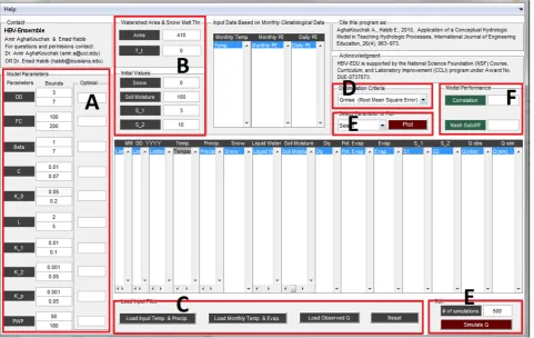
Figure 1 illustrates the HBV-Ensemble Graphical User In-terface (GUI). In panel a, the user can specify the upper and lower bounds of the parameters (see the first column in panel a). The initial values, such as the initial state of soil moisture, can be entered using panel b. Panel c can be used to load the input data. The required input data include precip-itation, temperature, long-term monthly evapotranspiration and temperature. Using panel d, the user can select the ob-jective function (e.g., root mean square error, Nash–Sutcliffe coefficient and correlation coefficient). The number of Monte Carlo runs (randomly sampled parameters) can be specified using panel e. Finally, the performance measure value for the simulation with the best performance value will appear in panel f.
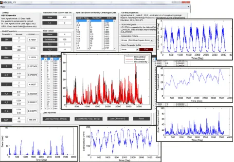
Figure 2 presents sample input precipitation (top), temper-ature (middle) and simulated ensemble streamflow (bottom). In Fig. 2 (bottom), the solid red line represents the observed runoff. The gray lines show the uncertainty limits for all the acceptable parameter value sets using 1000 simulations. In Fig. 2 (bottom) the solid black line displays the simulation from the best-estimate parameter-value set. One can see that in this approach, in addition to runoff, estimates of upper and lower bounds (gray lines) provide measures of uncertainty.
It should be noted that this educational toolbox produces other variables besides runoff, including time series of snow accumulation, soil moisture, evapotranspiration, and upper and lower reservoir water levels. For instance, Fig. 3 displays sample outputs derived using panel g in Fig. 1.
Fig. 1. HBV-Ensemble Graphical User Interface (GUI): (A) model parameters; (B) initial values and constants; (C) input data loading tools; (D) objective functions including root mean square error, Nash–Sutcliffe coefficient and correlation coefficient; (E) number of ensemble members; (F) model performance; (G) plotting tools.
Fig. 2. Top: input precipitation; middle: temperature; and bottom: simulated ensemble streamflow (simulated runoff – solid black line; observed runoff – solid red line; uncertainty space or ensemble sim-ulation – gray lines).
effects of initial values on streamflow simulation. For exam-ple, one can run the model with different initial values of soil moisture and compare the output hydrographs (as shown in Fig. 4). Using this particular exercise, student will find out that the initial values will have a significant impact on the model outputs at the beginning of the simulations. However, the effects of the initial values diminish over time in the long-term simulations.
[image:4.595.49.284.438.607.2]Fig. 3. HBV-ensemble sample model outputs (snow accumulation, soil moisture, evapotranspiration, and upper and lower reservoir water levels).
Fig. 4. Investigating the effect of initial value of soil moisture in streamflow simulation.
4 Students feedback and discussion
The previous version of the toolbox (Excel spreadsheet ver-sion) was used at the University of Louisiana at Lafayette (ULL) in Spring 2009 and students’ feedback were reported in AghaKouchak and Habib (2010). The presented educa-tional toolbox has been administered at the University of Cal-ifornia, Irvine (UCI) in Winter Quarters 2011 and 2012 (Wa-tershed Modeling CEE173-273). Students learned the fun-damentals of the HBV model concept and used the MAT-LAB GUI, shown in Fig. 1 for their final project (hydrologic modeling for a watershed in California). In the following, the feedback from UCI students who used the MATLAB GUI are presented.
[image:5.595.49.284.449.629.2]students who were exposed to this educational toolbox had already some background in hydrology.
In this course, the students are first exposed to the the-ory of the HBV model concept including calculations of snowmelt, snow accumulation, soil moisture, effective pre-cipitation, evapotranspiration, and runoff. During theoretical presentations of the course, with the help of the instructor, students perform all the calculations for a hydrologic mod-eling exercise in the class using an Excel spreadsheet. The reason for using a spreadsheet is to ensure students learn the calculations and how modeling works in general. This part of the course is designed to teach basics of hydrologic mod-eling, and does not include model calibration, validation and uncertainty. Once the students learn the fundamentals of hy-drologic modeling, the HBV-Ensemble, which includes pa-rameter sampling and calibration module, is presented in the class. With several homework assignments students practice model calibration, sensitivity analysis, the effects of initial conditions on model simulations, etc. For the final project, students are required to simulate the streamflow for a water-shed in California and submit a detailed project report.
In 2011 and 2012, a total of 60 students completed the project from which 56 students participated in an anonymous survey designed to gauge students’ learning gains. The sur-vey was administered once the students learned about the processes of HBV and how the toolbox works, but prior to completing the final project. Table 1 summarizes the survey questions. The first ten questions (Q1–Q10) aimed to gauge students’ learning gains as a result of using the presented ed-ucation toolbox. The last four questions (Q11–Q14) aimed to understand which aspects of this teaching tool contributed to students’ learning gains.
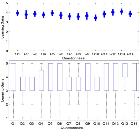
[image:6.595.309.546.61.279.2]Figure 5 presents students’ responses on their learn-ing gains uslearn-ing a five-point ranklearn-ing scale where: 1 = no gains; 2 = a little gain; 3 = moderate gain; 4 = good gain; and 5 = great gain. Figure 5 (top panel) displays the mean and confidence intervals (here defined as±3×the standard er-ror) of student responses for each question. Figure 5 (bot-tom panel) shows the boxplots of the students’ responses. On each box in Fig. 5 (bottom panel), the central red mark refers to the median, while the box edges are the 25th (25q) and 75th (75q) quantiles of the data. In the figure, the out-liers, defined as data points larger than 75q + 1.5 (75q−25q) or smaller than 25q−1.5 (75q−25q) (see McGill et al., 1978; Velleman and Hoaglin, 1981), are marked with a plus sign. The whiskers in Fig. 5 (bottom panel) represent the range of data points not considered outliers. Figure 5 indi-cates that this educational software had a positive impact on students understanding and knowledge of hydrological pro-cesses. Note that the students were asked to evaluate their learning gains as a result of their work with this education toolbox in the class (see Table 1). However, the authors ac-knowledge that evaluating students’ responses and associat-ing them to only the educational toolbox and not to the com-bination of instruction and model used was not possible in
Fig. 5. Students feedback (see Questions 1–15 in Table 1);
1 = no gains; 2 = a little gain; 3 = moderate gain; 4 = good gain; and 5 = great gain.
the current study. Furthermore, we acknowledge that a posi-tive student feedback does not necessarily prove the success of a teaching strategy and/or an educational approach, and it may only reflect a lumped assessment of the course.
It is worth repeating that the theoretical aspects of hy-drologic modeling were introduced prior to using HBV-Ensemble. The authors recommend using this educational toolbox after students are introduced to theoretical hydrol-ogy. Students, especially undergraduate students, without ba-sic knowledge of hydrology may not be able to benefit from this educational toolbox. Currently, efforts are underway to improve HBV-Ensemble by providing additional tools for teaching purposes. One example would be providing dotty plots, representing the best model parameterization and the parameter surface for each parameter versus the performance measure.
5 Conclusions
This study presents a modeling toolbox, HBV-Ensemble, de-signed for teaching hydrological processes, uncertainty anal-ysis, parameter estimation and model sensitivity to parame-ters and initial conditions. This modeling toolbox has been used in an upper level watershed modeling class at the Uni-versity of California, Irvine, and the students’ feedback have been positive as shown in Fig. 5.
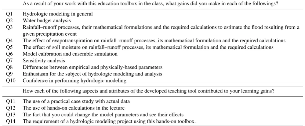
Table 1. Survey questions.
As a result of your work with this education toolbox in the class, what gains did you make in each of the followings?
Q1 Hydrologic modeling in general Q2 Water budget analysis
Q3 Rainfall–runoff processes, their mathematical formulations and the required calculations to estimate the flood resulting from a given precipitation event
Q4 The effect of evapotranspiration on rainfall–runoff processes, its mathematical formulation and the required calculations Q5 The effect of soil moisture on rainfall–runoff processes, its mathematical formulation and the required calculations Q6 Model calibration and ensemble simulation
Q7 Sensitivity analysis
Q8 Differences between empirical and physically-based parameters Q9 Enthusiasm for the subject of hydrologic modeling and analysis Q10 Confidence in performing hydrologic modeling
How each of the following aspects and attributes of the developed teaching tool contributed to your learning gains?
Q11 The use of a practical case study with actual data Q12 The use of hands-on calculations in the lecture
Q13 The fact that you could change the model parameters and see their effects Q14 The requirement of a hydrologic modeling project using this hands-on toolbox.
careers in hydrology. The presented modeling toolbox pro-vides the opportunity for students to investigate “what-if” scenarios for initial conditions, parameters, objective func-tions, etc., and practice experiential learning.
We recommend using HBV-Ensemble after students are introduced to theoretical aspects of hydrologic modeling. The toolbox can be used at the conclusion of an undergradu-ate hydrology class after the students have been already ex-posed to the fundamental processes; in such settings, the tool can serve as an add-on value for early introduction of ad-vanced concepts on model uncertainty and ensemble predic-tions. HBV-Ensemble can be used for in-class lab practices and homework assignments to improve students’ understand-ing of hydrological processes. Instructors, students and inter-ested readers can request a free copy of HBV-Ensemble for educational purposes.
Acknowledgements. The authors would like to thank the Editor
and reviewers for their constructive comments and suggestions which led to substantial improvements in the manuscript. We are grateful to many colleagues and graduate students who offered valuable comments and suggestions for improvements. These indi-viduals include Leonardo Valerio Noto, Ali Mehran, Jeff Tuhtan, Nasrin Nasrollahi, Mehdi Rezaeian Zadeh, Naveen Duggi and Mehdi Javadian. The first author acknowledges Andr´as B´ardossy’s classes and instruction approaches that inspired him to develop educational tools. Financial support from the United States Bureau of Reclamation (USBR) Award No. R11AP81451 to the first author and National Science Foundation Award No. DUE-1122898 to the third author are acknowledged.
Edited by: J. Seibert
References
AghaKouchak, A. and Habib, E.: Application of a conceptual hy-drologic model in teaching hyhy-drologic processes, Int. J. Eng. Educ., 26, 963–973, 2010.
AghaKouchak, A., B´ardossy, A., and Habib, E.: Copula-based un-certainty modeling: Application to multi-sensor precipitation es-timates, Hydrol. Process., 24, 2111–2124, 2010.
AghaKouchak, A., B´ardossy, A., and Habib, E.: Extremes in a Changing Climate, Springer, Dordrecht, The Netherlands, 2012. Bell, V. A. and Moore, R. J.: The sensitivity of catchment runoff models to rainfall data at different spatial scales, Hydrol. Earth Syst. Sci., 4, 653–667, doi:10.5194/hess-4-653-2000, 2000. Bergstr¨om, S.: The HBV model, Computer Models of
Water-shed Hydrology, in: Computer Models of WaterWater-shed Hydrology, edited by: Singh, V., Water Resources Publications, 443–476, 1995.
Beven, J. and Kimberlain, T.: Tropical Cyclone Report Hurricane Gustav (AL072008) 25 August–4 September 2008, Tech. rep., National Oceanic and Atmospheric Administration (NOAA), National Hurricane Center (NHC), USA, 2009.
Beven, K.: Environmental modelling: an uncertain future?, Tay-lor & Francis, 2008.
Beven, K. and Freer, J.: Equifinality, data assimilation, and uncer-tainty estimation in mechanistic modelling of complex environ-mental systems using the GLUE methodology, J. Hydrol., 249, 11–29, 2001.
Beven, K. J.: Rainfall-Runoff Modelling: The Primer, John Wiley and Sons, 2001.
Beven, K. J. and Binley, A. M.: The future role of distributed mod-els: model calibration and predictive uncertainty, Hydrol. Pro-cess., 6, 279–298, 1992.
Georgakakos, K., Seo, D., Gupta, H., Schaake, J., and Butts, M.: To-wards the characterization of streamflow simulation uncertainty through multimodel ensembles, J. Hydrol., 298, 222–241, 2004. Goodrich, D., Faures, J., Woolhiser, D., Lane, L., and Sorooshian, S.: Measurement and analysis of small-scale convective storm rainfall variability, J. Hydrol., 173, 283–308, 1995.
Habib, E., Ma, Y., Williams, D., Sharif, H. O., and Hossain, F.: Hy-droViz: design and evaluation of a Web-based tool for improving hydrology education, Hydrol. Earth Syst. Sci., 16, 3767–3781, doi:10.5194/hess-16-3767-2012, 2012.
Hundecha, Y. H. and B´ardossy, A.: Modeling of the effect of land use changes on the runoff generation of a river basin through parameter regionalization of a watershed model, J. Hydrol., 292, 281–295, 2004.
McGill, R., Tukey, J., and Larsen, W.: Variations of box plots, American Stat., 32, 12–16, 1978.
Montanari, A., Shoemaker, C., and van de Giesen, N.: Introduction to special section on Uncertainty Assessment in Surface and Sub-surface Hydrology: An overview of issues and challenges, Water Resour. Res., 45, W00B00, doi:10.1029/2009WR008471, 2009. Murphy, J., Sexton, D., Barnett, D., Jones, G., Webb, M., and Collins, M.: Quantification of modelling uncertainties in a large ensemble of climate change simulations, Nature, 430, 768–772, 2004.
Nash, J. E. and Sutcliffe, J. V.: River flow forecasting through con-ceptual models, Part I,. A discussion of principles, J. Hydrol., 10, 282–290, 1970.
NRC: Opportunities in the Hydrologic Sciences, National Academy Press, Washington, D.C., 1991.
NRC: Inquiry and the National Science Education Standards: A Guide for Teaching and Learning, National Academy Press, Washington, D.C., 2000.
Obled, C., Wendling, J., and Beven, K.: The sensitivity of hydro-logical models to spatial rainfall patterns: an evaluation using observed data, J. Hydrol., 159, 305–333, 1994.
Pathirana, A., Gersonius, B., and Radhakrishnan, M.: Web 2.0 collaboration tool to support student research in hydrol-ogy – an opinion, Hydrol. Earth Syst. Sci., 16, 2499–2509, doi:10.5194/hess-16-2499-2012, 2012.
Piani, C., Frame, D., Stainforth, D., and Allen, M.: Con-straints on climate change from a multi-thousand member ensemble of simulations, Geophys. Res. Lett., 32, L23825, doi:10.1029/2005GL024452, 2005.
Renard, B., Kavetski, D., Kuczera, G., Thyer, M., and Franks, S.: Understanding predictive uncertainty in hydrologic modeling: The challenge of identifying input and structural errors, Water Resour. Res., 46, W05521, doi:10.1029/2009WR008328, 2010. Rodhe, A.: Physical models for classroom teaching in hydrology,
Hydrol. Earth Syst. Sci., 16, 3075–3082, doi:10.5194/hess-16-3075-2012, 2012.
Rusca, M., Heun, J., and Schwartz, K.: Water management sim-ulation games and the construction of knowledge, Hydrol. Earth Syst. Sci., 16, 2749–2757, doi:10.5194/hess-16-2749-2012, 2012.
Seibert, J. and Vis, M. J. P.: Irrigania – a web-based game about sharing water resources, Hydrol. Earth Syst. Sci., 16, 2523–2530, doi:10.5194/hess-16-2523-2012, 2012a.
Seibert, J. and Vis, M. J. P.: Teaching hydrological modeling with a user-friendly catchment-runoff-model software package, Hy-drol. Earth Syst. Sci., 16, 3315–3325, doi:10.5194/hess-16-3315-2012, 2012b.
Shaw, S. B. and Walter, M. T.: Using comparative analysis to teach about the nature of nonstationarity in future flood predictions, Hydrol. Earth Syst. Sci., 16, 1269–1279, doi:10.5194/hess-16-1269-2012, 2012.
Singh, V. and Woolhiser, D.: Mathematical Modeling of Watershed Hydrology, J. Hydrol. Eng.-ASCE, 7, 269–343, 2002.
Thompson, S. E., Ngambeki, I., Troch, P. A., Sivapalan, M., and Evangelou, D.: Incorporating student-centered approaches into catchment hydrology teaching: a review and synthesis, Hy-drol. Earth Syst. Sci., 16, 3263–3278, doi:10.5194/hess-16-3263-2012, 2012.
Velleman, P. and Hoaglin, D.: Applications, basics, and comput-ing of exploratory data analysis, vol. 142, Duxbury Press Boston, Boston, 1981.
Vrugt, J. A., ter Braak, C. J. F., Clark, M. P., Hyman, J. M., and Robinson, B. A.: Treatment of input uncertainty in hy-drologic modeling: Doing hydrology backward with Markov chain Monte Carlo simulation, Water Resour Res., 44, W00B09, doi:10.1029/2007WR006720, 2008.
Wagener, T.: Evaluation of catchment models, Hydrol. Process., 17, 3375–3378, 2003.
Wagener, T., Wheater, H., and Gupta, H.: Rainfall-runoff modelling in gauged and ungauged catchments, Imperial College Press, London, UK, 2004.
Wagener, T., Sivapalan, M., Troch, P. A., McGlynn, B. L., Har-man, C. J., Gupta, H. V., Kumar, P., Rao, P. S. C., Basu, N. B., and Wilson, J. S.: The future of hydrology: An evolving sci-ence for a changing world, Water Resour. Res., 46, W05301, doi:10.1029/2009WR008906, 2010.
Wagener, T., Kelleher, C., Weiler, M., McGlynn, B., Gooseff, M., Marshall, L., Meixner, T., McGuire, K., Gregg, S., Sharma, P., and Zappe, S.: It takes a community to raise a hydrologist: the Modular Curriculum for Hydrologic Advancement (MOCHA), Hydrol. Earth Syst. Sci., 16, 3405–3418, doi:10.5194/hess-16-3405-2012, 2012.
Wheater, H. S., Jakeman, A. J., and Beven, K. J.: Progress and di-rections in rainfall-runoffmodelling, in: Modelling change in en-vironmental systems, edited by: Jakeman, A. J., Beck, M. B., and McAleer, M. J., Wiley, 1993.
Wood, A., Maurer, E., Kumar, A., and Lettenmaier, D.: Long-range experimental hydrologic forecasting for the eastern United States, J. Geophys. Res.-Atmos., 107, ACL6-1-15, doi:10.1029/2001JD000659, 2002.