WRL 89 14 pdf

WRL

Research Report 89/14

Long Address Traces

from

RISC Machines:

Generation

and

Analysis

research relevant to the design and application of high performance scientific computers. We test our ideas by designing, building, and using real systems. The systems we build are research prototypes; they are not intended to become products.

There is a second research laboratory located in Palo Alto, the Systems Research Cen-ter (SRC). Other Digital research groups are located in Paris (PRL) and in Cambridge, Massachusetts (CRL).

Our research is directed towards mainstream high-performance computer systems. Our prototypes are intended to foreshadow the future computing environments used by many Digital customers. The long-term goal of WRL is to aid and accelerate the development of high-performance uni- and multi-processors. The research projects within WRL will address various aspects of high-performance computing.

We believe that significant advances in computer systems do not come from any single technological advance. Technologies, both hardware and software, do not all advance at the same pace. System design is the art of composing systems which use each level of technology in an appropriate balance. A major advance in overall system performance will require reexamination of all aspects of the system.

We do work in the design, fabrication and packaging of hardware; language processing and scaling issues in system software design; and the exploration of new applications areas that are opening up with the advent of higher performance systems. Researchers at WRL cooperate closely and move freely among the various levels of system design. This allows us to explore a wide range of tradeoffs to meet system goals.

We publish the results of our work in a variety of journals, conferences, research reports, and technical notes. This document is a research report. Research reports are normally accounts of completed research and may include material from earlier technical notes. We use technical notes for rapid distribution of technical material; usually this represents research in progress.

Research reports and technical notes may be ordered from us. You may mail your order to:

Technical Report Distribution

DEC Western Research Laboratory, UCO-4 100 Hamilton Avenue

Palo Alto, California 94301 USA

Reports and notes may also be ordered by electronic mail. Use one of the following addresses:

Digital E-net: DECWRL::WRL-TECHREPORTS

DARPA Internet: [email protected]

CSnet: [email protected]

UUCP: decwrl!wrl-techreports

Generation and Analysis

Anita Borg, R. E. Kessler, Georgia Lazana, and David W. Wall

The accurate analysis of cache designs is becoming ever more important as processor speeds rapidly outstrip memory speeds and cache misses become a more significant factor in system performance. It can easily be shown that a factor of 10 decrease in processor cycle time with no change in the memory system may increase execution speed by only a factor of 2, the difference be-ing due only to the increased relative cost of servicbe-ing cache misses.

The primary tool for cache analysis is simulation based on address traces of running systems. The accuracy of the results depends both on the simula-tion model and the accuracy of the trace data. Existing methods of generat-ing and analyzgenerat-ing traces suffer from a variety of limitations includgenerat-ing com-plexity, inaccuracy, lack of system references, short length, inflexibility, or applicability only to CISC machines.

We have built a system for generating and analyzing traces that addresses each of these problems. Trace generation is based on link-time code modification that makes the generation of a new trace easy. The slowdown of trace-linked code is small enough to allow reasonably accurate traces of user/system interaction. The system is flexible enough to allow great control of what is traced and when it is traced. On-the-fly analysis removes most limitations on the length of traces. The system is designed for use on RISC machines.

In this paper we describe the implementation of trace generation and on-the-fly analysis. We then review preliminary results from the analysis of user traces containing many billions of memory references. Very long traces are both useful and necessary for understanding the behavior of large, fast systems. We experiment with overall size, block size, and associativity in second level caches.

1.1. Background

For 20 years traces of memory access patterns have provided a window into program execu-tion, allowing the simulation of memory systems with the goal of evaluating different cache designs [14]. The analysis of cache designs is becoming even more crucial as caches become dramatically faster than main memory and cache misses are an ever more important factor in system performance. For example, on today’s RISC machines, it typically takes ten times longer to retrieve data from main memory than from the cache, whereas on machines currently being designed the ratio will be 100 to 1. Many new processor designs use RISC technology with very fast on-chip caches. Since it is infeasible to put sufficiently large caches on chip, somewhat slower, but very large, off-chip second level caches will be used to improve performance. Second Level caches of 16 megabytes or more may sit between the processor and a gigabyte of main memory.

Simulation is the primary tool for determining the appropriate sizes and characteristics of memory systems for the new RISC machines. To be able to accurately simulate the behavior of very large caches, very long RISC traces are needed. We are unaware of any existing traces that represent more that O(10 million) memory references. Existing traces are usually sufficient for the simulation of small caches on CISC machines, but they are too short to simulate multi-megabyte caches. We also believe that RISC traces are sufficiently different from CISC traces to warrant the generation of fresh traces. RISC code for a program is often twice as large as corresponding CISC code, increasing the number and range of instruction references. Also, ef-fective use of the large register sets built into RISC machines reduces the number of data references compared to code for a CISC machine. At the very least, the balance of instruction and data references will change markedly.

Unfortunately, existing methods are inappropriate for generating long traces and for use on RISC machines. The most common software method involves the simulation of a program’s execution to record all of its instruction and data references. This method is both slow and limited. Simulation is slow for CISC programs and may be slower for RISC programs because they contain more instructions each requiring a pass through the main simulator loop. A 1000x or more slowdown makes traces of real-time behavior, including kernel and multiprogrammed execution, impossible to accurately simulate. Some hardware methods spy on address lines to trace execution in real time, but these usually have limited capacity. In ATUM [1], trace genera-tion involves microcode modificagenera-tion. The microcode for a machine is modified to trap address references and generate trace data. A microcode-modified machine runs only 10 times slower than an untraced machine. The method is not applicable to RISC machines since there is no microcode to be modified.

At WRL, where we design, build, and use high performance RISC machines, we have developed a method of trace generation that is appropriate for use on those machines. We make use of link-time code modification to generate code that will create a record of data and instruc-tion references. Both user and operating system execuinstruc-tion can be traced with 8 to 12x slow-down. On-the-fly trace analysis, in which trace data is analyzed as it is collected, eliminates the need to store traces and makes the analysis of very long traces feasible.

1.2. Goals and Status

The primary goal of this project is to implement a set of tools for trace generation on RISC machines, and to use them to analyze the memory system designs for our next machine. We require that:

•The traces must be complete. They must represent kernel and multiple users as they execute on a real machine. The memory references must be interleaved as they are during execution rather than being artificially interleaved separate traces.

•Traces must be accurate. The mechanism used must not slow down execution to the extent that the behavior of the system is no longer realistic.

•Tracing must be flexible. We must be able to pick and choose the processes to be traced, optionally trace kernel execution, and turn tracing on and off at any time. •The traces must be long enough to make possible the realistic simulation of very

large caches.

A new trace generation mechanism can satisfy the first three requirements, but new analysis techniques are required to meet the fourth. Since the trace lengths we require can outstrip storage capacity, analysis that is done off-line against stored traces is unacceptable. Therefore our research extends into methods of managing and analyzing long traces.

Initially, the traces will be used to analyze the behavior of multi-level cache hierarchies in very fast machines. Eventually, we will be interested in exploring other uses for the traces we generate. For example, Sites [1, 13] has had considerable success in using his traces as a debug-ging tool that gives a much more detailed picture of program execution than does profiling infor-mation. McFarling [10] discusses the use of profiling information to place code for cache op-timization. Traces may also be a useful tool for determining code placement.

2. Trace Generation

2.1. Environment: The Titan

The original RISC machine designed and built at WRL was the Titan. It is currently our primary workhorse and the machine whose execution we have traced. The Titan is an ex-perimental, high performance, 32-bit RISC workstation with a 45ns cycle time, different register sets for user and kernel, and a maximum memory configuration of 128 megabytes. A program may reference 64 general purpose registers. Titans run a modified version of Ultrix called



Tunix (Titan Unix ) in which all process and memory management functions have been rewrit-ten.

2.2. Link-time Code Modification

Our trace generation method relies on the ability to do link-time code modification. All com-pilers at WRL translate programs into an intermediate language, Mahler, which defines the abstract machine, hiding the details of the hardware from the compilers. The Mahler implemen-tation [17, 18] consists of a translator and an extended linker. Object modules produced by the Mahler translator contain sufficient supplementary information to allow the linker to do global register allocation and pipeline scheduling, as well as the code modification we require for trace generation. In particular, basic blocks and their sizes are identifiable at link-time.

An option to the linker causes branches to trace code to be inserted in the program wherever a referenced address is to be recorded. A return address is saved in a reserved register, thereby avoiding a complex call/return mechanism. Trace code uses reserved registers to access its ar-guments so that memory accesses are minimized. When executed, the trace code computes a virtual address (physical address for the kernel) and writes the address in a trace buffer. An instruction address computed and written into the trace buffer is the address at which the instruc-tion would have been located had the code not been expanded with trace branches. A trace resulting from the execution of trace-linked code represents an execution of normally linked code. An example of the effect of code expansion follows:

Original code:

(addr1) lab1: r1 := 4[r2] r1 := r1 + 1 8[r2] := r1

if r1>0 goto lab2 null

Expanded Code (symbolic):

lab1: call InstrTrace(5,addr1) call LoadTrace(ADDR(4[r2])) r1 := 4[r2]

r1 := r1 + 1

call StoreTrace(ADDR(8[r2])) 8[r2] := r1

if r1>0 goto lab2 null

call InstrTrace(7,addr2) r1 := r9 + r10

...

where ADDR(d[rn]) means the address in memory described by displacement d and the contents of base register rn.

Expanded Code :

lab1: r48 := pc, goto InstrTrace r49 := 5

.word (addr1)

r48 := pc, goto LoadTrace r50 := loadaddr 4[r2] r1 := 4[r2]

r1 := r1 + 1

r48 := pc, goto StoreTrace r50 := loadaddr 8[r2]

8[r2] := r1

if r1>0 goto lab2 null

r48 := pc, goto InstrTrace r49 := 7

.word (addr2) r1 := r9 + r10 ...

2.3. Operating System Support

The operating system’s primary trace-related job is the management of the trace buffer. The trace must reflect the actual sequence of memory references made by a mixture of user and ker-nel programs. Therefore, the trace buffer is shared among the kerker-nel and all running processes. Only those processes that have been linked for tracing actually use the buffer.

At boot time, the trace buffer is allocated from the free page pool. The current system runs on a Titan with 128 megabytes of memory. The trace pages are permanently associated with the trace buffer and are not pageable. During execution, the machine behaves as if it had less physi-cal memory. We have experimented with 32 and 64 megabyte trace buffers.

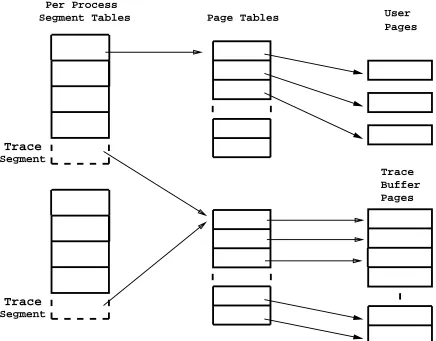
From within the operating system, the buffer is referenced directly using its physical ad-dresses. To make user references to the trace buffer sufficiently fast, the buffer is mapped into the high end of every user’s virtual address space, as shown in Figure 1.

Segment Tables Per Process

Page Tables

Pages User

Trace Buffer Pages

Trace

Segment

Trace

Segment

Figure 1: Mapping of the shared trace buffer

process has text, initialized data, uninitialized data and stack segments. The trace pages make up a shared fifth segment. The stack, which usually resides at the high end of the 1 gigabyte virtual address space, is moved to below the trace buffer. The address space is large enough that this does not constrain user programs. Since a single trace segment with its page table is set up at boot time to be shared by all processes, the operations required on creation of a new process are minimal, involving only the copy of a pointer to the segment.

2.4. The Trace Code

For efficiency, the trace code itself was written in TASM (Titan Assembly Language) using registers to avoid memory references. The only memory references in the trace code are writes to the trace buffer. All other values needed to manage tracing (pointer to the next available trace location, value to be written, return address, trace flag, etc.) are kept in registers. A simple branch instruction is used to return from the trace code. In user programs, 18 TASM instructions are executed to generate a data trace and 22 to generate an instruction trace. In the kernel, 14 and 18 are executed, respectively.

A Titan register set contains 64 general purpose registers, 58 of which are normally available to user programs. We use 8 of these registers for trace generation. As a result, the operating system and code linked for tracing each have 50 registers available.

The kernel uses a separate register set from user processes. To assure that the trace registers are always correct, some of their values must be copied back and forth between register sets when moving between user and kernel mode. On every transfer from one register set to another, two values (the current buffer index and buffer pointer) must be copied from one register set to the other via memory. If the transfer is between a kernel register set and a user register set the buffer pointer is not copied, but is recalculated from the index and virtual or physical buffer base address as appropriate. The translation to a virtual address is the same for all processes since the buffer resides at exactly the same virtual address in all processes.

Kernel execution on the Titan is uninterruptible, however, user execution can be interrupted at any time, in particular in the midst of trace code. This complicates the trace code and the code executed on entry to and exit from the kernel. Additional code must assure correct synchroniza-tion among the users of the trace buffer. Since interrupts can occur between arbitrary instruc-tions, a lock value (requiring a register) is used to indicate that a user was interrupted mid-trace and that the kernel must take special action. The kernel’s trace registers must be made consis-tent, and the user’s registers must be properly restored to continue mid-trace on return from ker-nel mode. This complication accounts for the difference in length between the kerker-nel and user trace code. The only inelegant result of this is that a user trace entry can be split, with an ar-bitrary amount of trace data generated by the kernel or other users in between the two parts of the entry.

2.5. Controlling Tracing

Tracing is done only when a trace flag kept in one of the trace registers is turned on. Before writing to the trace buffer, the value of the trace flag if checked. If it is off, control returns to the program without writing to the trace buffer. Tracing is turned on at the first interrupt following a write to a location in /dev/kmem, a UNIX device corresponding to kernel memory that allows privileged users to modify kernel values. Tracing is turned off in an analogous fashion.

When tracing is off, 4 to 6 additional instructions are executed at every trace point. No ad-ditional cost is incurred during the execution of user code that is not linked for tracing whether or not tracing is turned on. The modified kernel, even when not linked for tracing, is slower by a factor of about 2 because even a non-traced kernel must do extra work on every kernel entry to assure that the trace registers are kept consistent.

2.6. Explicit Trace Buffer Entries

In addition to the automatic generation of address reference information as the result of linker inserted branches, it is possible to explicitly call trace routines from either the user or the kernel to insert arbitrary informative items into the trace. Currently we make use of this in the kernel.

The addresses inserted in the trace buffer by the kernel are physical addresses, whereas those inserted by user processes are virtual addresses. It is essential for the analysis code to be able to tell one from the other. It is also useful to be able to associate sequences of virtual addresses with a particular process when more than one is being traced. Therefore, on every transfer into or out of the kernel a change mode entry is made in the trace buffer. The entry indicates whether the change is from user to kernel or kernel to user and which user process is involved.

2.7. Format of Trace Buffer Entries

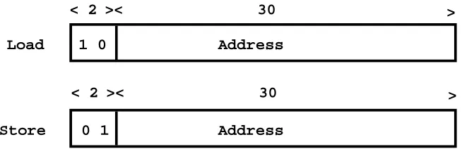
Entries in an address trace can be divided into two types based on whether they fill one or two 32-bit words of the trace buffer. Data reference entries, the majority of all entries, are one word long. All others are two words long. An address generated in kernel mode is physical. An address generated in user mode is virtual.

Data Load/Store entries take up a single 32-bit word. Since we trace word addresses from a 1 gigabyte address space, the two high order bits are always available as a type field. Any trace entry with non-zero high order bits is a data entry. The first word of other types of entries contain type information in the high order byte.

Load Address

Address Store

1 0

0 1

< 2 >< 30 >

< 2 >< 30 _>

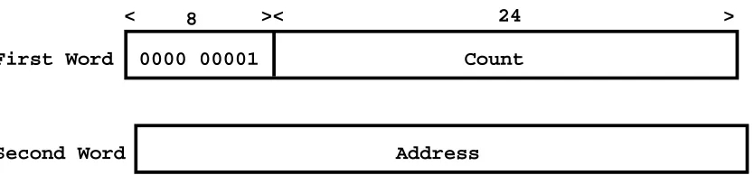
An Instruction entry represents the beginning of a basic block. The essential characteristic of a basic block is that all instructions in the block are presumed to execute sequentially.

< >< >

0000 00001 Count

24 8

First Word

Address Second Word

Figure 3: Instruction entry format

Count is the number of instructions in the basic block starting at the address in the second word.

2.8. Kernel Tracing: A Few Special Considerations

Our goal is to be able to relink the kernel just as we do a user program in order to trace its execution. This is possible for nearly all kernel code, with the exception of a portion written in TASM and never modified by the linker. This section corresponds to the very low level machine-dependent code in Unix and is currently not traced. In Tunix, the code determines the cause of traps and interrupts, saves and restores coprocessor state and process state (register contents), manipulates the clock and translation look aside buffer (TLB), and manages returns from interrupts. It also includes the idle loop. We will eventually want to trace the TASM code. To do this, calls to trace routines will be selectively inserted into the code (all but the idle loop) by hand.

3. Trace Management

3.1. Extracting the Traces from Memory

The system as described thus far can very quickly gather an address trace whose length is the size of the trace buffer. Tracing slows execution by about 8 to 12 times. Even with a 64 megabyte trace buffer (half of the Titan’s memory), the trace represents only about 2 seconds of untraced Titan execution time or 30 to 35 million memory references. While such traces are much longer than those commonly available and are interesting for some purposes, they are not nearly long enough to analyze the behavior of a very large cache. This means that the trace data must be extracted from the buffer in such a way that execution can continue without too much disruption, in particular, without affecting the accuracy of the trace data.

Neither extraction nor analysis of the data can be done simultaneously with tracing because either is orders of magnitude slower than trace generation. Thus, all methods of dealing with long traces require that tracing be periodically interrupted for a significant amount of time. The challenge is to assure that the resulting traces are seamless, that is, that they reflect address refer-ence patterns that would have occurred had the machine continued tracing without interruption.

analyzed immediately, eliminating the need to save the trace. The first possibility does little to solve the ultimate problem of very long traces where storage is impractical or impossible. Trac-ing of 5 minutes of Titan execution could generate nearly 10 gigabytes of uncompressed trace data.

While we have implemented a mechanism to extract, compress, and write partial traces to high density tape, our preferred method is to analyze the trace data on the machine being traced as it is generated. When the trace buffer becomes nearly full, the operating system turns off tracing and runs a very high priority analysis process. As with any other process running on the traced machine, the trace buffer is mapped directly into the analysis program’s address space so that the data can be directly accessed.

Execution of the analysis program is controlled by the use of a read system call on a special file. The program opens the file and attempts to read it. The read returns the virtual address of the beginning of the trace buffer and the number of available entries only when the buffer is full (or nearly full). The program may then do anything it chooses with the trace data. The operating system guarantees that during the execution of the analysis program, tracing is turned off and traced programs are not scheduled for execution.

When all current data in the buffer has been processed, the special read is once again ex-ecuted, tracing is turned back on, and traced user programs can once again execute.

3.2. Reproducibility of Results

A valuable characteristic of stored traces is the reproducibility of simulation results. When traces are generated and stored for later use, the identical trace can be used to simulate and com-pare different cache organizations. On-the-fly analysis does not provide that capability. While sub-traces of executions of any single deterministic user program will be identical, the inclusion of multiple processes will cause traces to vary from one run to the next. Likewise, kernel traces will never be identical from run to run.

There are a couple of potential solutions to this problem. First, it might be possible to simu-late more than one cache organization at a time. The utility of this approach is clearly limited because it does not allow old results to be compared with new ones. Another possibility is to do a sufficient number of controlled runs to determine the variance in results for each cache or-ganization so that any statistically significant difference between two different caches organiza-tions can be determined. While this is more painful and time consuming than either stored traces or multiple simultaneous simulation, the results will more accurately represent the reality of ex-ecution on an actual machine.

4. Accuracy of the Trace Data

tracing, and the interruption of traced programs in order to execute trace extraction and analysis code.

4.1. Eliminating Gaps for Seamless Traces

For a trace to accurately represent real execution, there must be no gaps in the trace. One cause of such gaps can be the interruption in tracing during trace extraction and analysis.

If only user programs that are not time dependent are traced, seamlessness is not an issue. Traced users are excluded from execution while the analysis program is run and resume execu-tion at precisely the point they were stopped once the trace buffer has been emptied. Since the cache simulation analysis we do takes approximately two orders of magnitude more time than does execution of the traced code, time dependent programs will behave very strangely, if they work at all.

The effect of analysis breaks is more difficult to deal with when the kernel is traced. The kernel cannot be prevented from executing while the analysis program runs and tracing is turned off. While it is not appropriate to trace kernel operations that are executed on behalf of the analysis program, the trace should include code that services interrupts belonging to the traced process, such as the completion of I/O initiated by a traced user process.

Careful placement of the code that turns off tracing prior to running the analysis program as-sures that the trace sequence is a realistic one that could have actually occurred in the absence of tracing. We have not yet come up with a solution to missing interrupt traces. For the moment, we will analyze the problem to understand how often this happens and to determine the effect on the accuracy of the analytical results.

4.2. Trace-Induced TLB Faults

The second type of inaccuracy occurs when code is traced that is solely an artifact of tracing. Since the only extra code executed in user mode is the trace code itself, which is not traced, this inaccuracy occurs only during kernel tracing.

For example, a TLB fault that would not occur during the execution of untraced code is generated whenever a user process first references a new page of the trace buffer. Since TLB faults are handled in software in the kernel, a kernel trace would contain a record of the execu-tion of the TLB fault handler. If the trace of the fault handler were sufficiently long, the next user reference to the trace buffer could be to the next page of the buffer and could generate another TLB fault. Execution would thrash in a nasty loop filling the trace buffer only with fault execution traces. This situation did occur during the early debugging of the system. Note that references to the trace buffer never cause page faults because the buffer is locked into memory.

the I/O interrupt. Our solution is to modify the low level TASM interrupt code in the kernel to detect this situation and turn off tracing whenever a TLB fault on an address in the range known to be the trace buffer occurred, and to turn it on again on return to user mode or if additional work is to be done prior to returning to user mode.

Another cause of trace induced TLB faults is the modification of the tlb during trace extraction and analysis. Execution of the analysis code and references to many trace buffer pages are guaranteed to substantially modify the TLB. After the analysis program has run, the traced user process would normally have to re-fault in its relevant translations. To solve this, we may save the contents of the TLB after turning off tracing but before running the analysis program. The contents of the TLB are then restored prior to turning tracing back on.

4.3. Interrupt Timing

Traces may not accurately represent normal execution because code segments are executed at a different time, i.e. in a different order, when tracing is on. Any slowdown in execution means that various interrupts happen sooner or more frequently than they would without tracing. This will affect traces for user code that does asynchronous I/O or relies on signals. I/O will appear to be considerably faster because less user code (and more trace code) is executed between initia-tion and compleinitia-tion of an I/O operainitia-tion. We consider this distorinitia-tion a necessary evil.

Also problematic are the additional timer interrupts that are not only traced (in kernel mode) but affect the rate at which process switching is mandated. This effects the scheduling of user processes because less code will be executed before a single process’s time quantum runs out. This can be fixed by changing the quantum associated with traced processes. If the effect of additional timer interrupts in kernel traces turns out to be problematic, it will have to be ac-counted for in the analysis program rather than by modifying the traces.

4.4. Process Switch Interval

The decreased execution speed for traced processes influences the accuracy of multiple process traces. Since the process switch interval is measured in time rather than instructions, the number of original instructions executed between process switches is 8-12 times less than nor-mal. If such traces are used to simulate cache behavior, the resulting performance will be er-roneously low. To account for this we increased the process switch interval. This was done without changing the interval at which clock interrupts were serviced to check for external inter-rupts since interinter-rupts still need to be recognized quickly.

Initially, we increased the process switch interval by a factor of 8 to reflect actual switching on a Titan. This corresponds to the execution of approximately 200,000 user instructions between switches. Since we are interested in simulating machines that are faster than the Titan we also experimented with an interval corresponding to 400,000 instructions between switches. We do not know of any other multiprocess trace generation system which attempts to take this into ac-count.

measured in cycles rather than in instructions. With no stalls, the Titan would issue one instruc-tion per cycle, but it does not run at that rate. Also, only compute bound programs regularly use their entire time quantum on each switch.

5. Verification

It is difficult to verify the absolute correctness of many gigabytes of trace data, however, we were able to use a number of techniques to convince ourselves of their accuracy.

5.1. Comparison with Simulation Results

An instruction level simulator existed for the Titan. The simulator already produced cache hit and miss data and was modified to produce traces for short, but real, user programs. For ease of comparison, our regular cache analysis program was modified to write out traces in exactly the form produced by the simulator. The resulting trace files were compared and the number of cache hits and misses were compared.

The differences we noted first exposed bugs and then showed some surprising cache perfor-mance results that would not have been obvious using only one trace method. While instruction addresses matched, we were puzzled by differences in data addresses and data cache hit rates. It turned out that the simulator made different assumptions about the virtual address at which the user process’s stack began from that made by the operating system. This affected the cache locations used by stack references. The surprising result was that this small change resulted in as much as a 15% difference in the hit rate in the data cache.

While the simulator could not be used to simulate kernel details, it was still extremely useful. We were able to verify that the trace sequence was correct and that the addresses computed in the trace code corresponded to the correct addresses referenced by executing code that was not expanded for tracing. Since the link-time modification is the same for user and kernel code, we believe that this justifies confidence in the accuracy of both kernel and user traces.

5.2. Checking for Gaps

In addition to checking the correctness of the information created by the trace code, it was necessary to assure that kernel and user accesses to the trace buffer were properly synchronized, and that no gaps in traces were produced when the analysis program ran.

Two techniques were used to verify correct synchronization. First, we traced a program that infinitely executed a very simple tight loop, thus generating an easily recognizable pattern, and then ran a variant of the analysis program that checked whether anything was missing or out of place.

6. Trace Analysis

6.1. Panama: A Cache Analysis Program

Panama is our first and most general cache analysis program. The requirements were that it be flexible and easily modifiable so that cache characteristics could be changed from run to run. The program should take up as little space as possible so that we can run large user programs without additional paging overhead. Since analysis is the slowest part of the process taking easily 10 times as long as trace generation, it should be as fast as possible.

To achieve speed and small size, we sacrificed run-time flexibility and were satisfied with compile-time flexibility. Constants whose values are specified at compile-time define the fol-lowing cache characteristics:

•Number of cache levels (1 or 2)

•Split or integrated data and instruction caches •Degree of associativity

•Number of cache lines •Line size

•Write policy (write through or write back)

•Cost of hit and miss (in units of processor cycles)

A version of the program is compiled for each cache configuration, thus minimizing space allocated for run-time data structures and eliminating code that is not executed for that con-figuration. Panama can also simultaneously simulate a fully associative version of the second level cache.

Output of the trace analysis is generated at intervals that can be based on the number of structions, trace entries, or memory references encountered. The data written includes both in-terval and cumulative summaries of the following information:

•For each cache:

•number of references

•miss ratio

•contribution to the cycles per instruction (CPI_cache)

•the percent of misses that resulted from user/kernel conflicts

•Contribution to the CPI by second level cache compulsory misses (first time references)

•Second level cache contribution to the CPI if fully associative •For user mode and kernel mode:

•Number of cycles executed and CPI

Panama works well, but remains a candidate for speed optimization. When simulating split instruction and data first level caches and a direct-mapped second level cache, analysis plus trace generation take about 100 times as long as untraced execution. For example, tracing and analyz-ing a run of TV, a WRL timanalyz-ing verification program, extends the run time from 25 minutes to 45 hours.

6.2. Tycho: Evaluating Associativity

Tycho is a cache simulation program developed by Mark Hill [6] that allows many different single level cache configurations to be simulated concurrently. The algorithm used is the special case of all-associativity simulation [9]. Although our primary interest is with multi-level caches, we used Tycho to determine whether very long traces produced different results than short traces and whether such effects varied with the degree of associativity.

6.3. Saving Traces for Later Analysis

On-the-fly analysis techniques allow us to analyze traces of unlimited length, but the need for long traces outside of WRL convinced us to generate and save a set of traces for distribution. Data storage was the primary problem to be overcome. We decided to put the data on tape for



two reasons: capacity and portability. Sony 8mm video cartridges used with an Exabyte drive chosen for their large storage capacity, 2 gigabytes, and their convenience. The cartridges are the size of a normal audio cassette tape.

Techniques similar to the Maching scheme used in [12] were used to pack massive amounts of trace data on each tape. The original trace data is first converted into a cache difference trace consisting of reference points and differences. Addresses are represented as the difference from a previous address, rather than as an absolute address. This differencing creates many repeated patterns in the trace reference string. The cache difference trace is then run through the Unix

compress program. Compress uses Lempel-Ziv [20] compression to recognize common

se-quences of data and compress these sese-quences into single code words. Reference locality and the regularity of trace entry formats allows trace data to be very effectively compressed. We were able to reduce the storage requirements to between 0.38 and 3.0 bits per memory reference, with most traces in the 2-3 bit range. This allowed us to store a trace of about 8 billion memory references on a single tape.

7. Experiments with Single and Multiple Process User Traces

7.1. Base Case Cache Organization Assumptions

A number of assumptions have been made about the type of machine we are interested in analyzing. They are based on discussions with WRL’s hardware engineers and represent some broadly accepted projections for workstations of the future. The assumptions define the basic cache organization whose characteristics we then varied and simulated.

instruction types other than loads and stores. The remaining assumptions are built into the Panama analysis program.

We assume a pipelined architecture where, in the absence of cache misses, a new instruction is started on every cycle. This is possible when the page offset is simultaneously used to retrieve the real page from the TLB and to index the correct line in the cache. Since we do not consider delays other than those caused by cache misses, we count the base cost of instruction as one cycle. The goal of the memory hierarchy design is to keep the CPI as close to 1 as possible.

We also assume the machine is fast enough to require two levels of cache. The additional cost of going to the second level cache, in case of a miss in the first level cache, is assumed to be 12 cycles. This is the same as the cost of going to main memory on a Titan. The cost of going to main memory is assumed to be 200-250 cycles depending on the size of block that is retrieved.

The first level data cache is presumed to be a write through cache with an associated write buffer. In our experiments, the capacity of the write buffer is 4 entries. If there is a entry avail-able, the write occurs at no additional cost, otherwise the write stalls. An entry is retired, that is, it commits in the second level cache and frees space in the write buffer, every 6 cycles. In other words the write buffer behaves like a 4-entry FIFO, queuing up the writes to the second level cache.

The second level cache is write back. It may be either virtually or physically addressed. We have used a mapping based on virtual user addresses and physical kernel addresses. It is described in detail in Section 7.5.

7.2. Choice of User Programs

Our choice of user programs to trace is based upon the assumption that in the future machines will have much larger memories and that programs will be written to use that memory. Ideally, the programs should characterize the average workload of a future system. Unfortunately, an "average" workload is difficult to define. Not only are there wide variations in use from one user to another, but the usage changes with time. Prediction of a future workload is a difficult problem. We are confident of one thing. Applications will grow to use the large amounts of memory available in future machines.

Most programs today have working sets of less than 16 megabytes. Some programs have large address spaces but only use very small portions at a time to avoid thrashing on small memory machines. Nearly every program we have chosen to trace is real and currently in use on existing large machines. Many are memory hogs by today’s standards, but not simply because they are poorly written. They require large amounts of memory because the problems they are solving are inherently large.

Figure 4 describes the programs we have traced thus far. In the remaining sections we will focus on the following four examples.

•TV is a timing verifier for VLSI circuits which is in regular use at WRL. It

Traced User Programs

Name Description

Make Unix program to maintain, update, and regenerate groups of programs. The make program was used to generate a sequence of compiles and loads. It made calls to cc, rm, and cat.

Cc C compiler front end. It initiates the C pre-processor, C compiler, Mahler compiler, and loader.

Cpp C language preprocessor.

Ccom First phase of C compilation on the Titan.

Mc Titan Mahler [18] intermediate language compiler.

Xld Titan extended linker and loader.

Cat Unix utility to concatenate files.

Cp Unix utility to copy files.

Vi/Ex Unix text editor.

Ps Unix utility to read process status.

Ls Unix utility to list directory contents.

rm Unix utility to remove a file.

Tcsh Unix shell program.

Magic VLSI editor [11]. It has a number of features not found in other editors, including design rule checking, plowing, etc.

Grr Printed circuit board router [4].

TV Circuit timing verifier [7].

SOR Fortran implementation of the successive overrelaxation algorithm [3, 8] that uses sparse matrices.

Linear Program to solve linear systems of equations using sparse matrices [15].

Tree Compiled Scheme program which builds a tree data structure and searches for the largest element in the tree [2].

Figure 4: Descriptions of programs used in trace experiments

•SOR executes Renato De Leone’s implementation of the successive overrelaxation

algorithm using sparse matrices. It is written in Fortran with static array allocation. It operates on a 800,000 by 200,000 sparse matrix with approximately 4 million (0.0025%) non-zero entries and takes 62 Mbytes.

•Tree is a compiled Scheme program, written by Joel Bartlett, which builds a tree

•Mult is a multiprogramming workload consisting of:

•a make run compiling (from C) portions of the Magic source code

•grr routing the DECstation 3100 printed circuit board

•Magic design rule checking the MultiTitan CPU chip

•Tree on a smaller problem given 10Mbytes of working space

•another make run that calls xld on the Magic code

•an infinitely looping shell of interactive commands (cp, cat, ex, rm, ps -aux, and ls -l /*)

This set of programs uses approximately 75 Mbytes of memory.

iiiiiiiiiiiiiiiiiiiiiiiiiiiiiiiiiiiiiiiiiiiiiiiiiiiiiiiiiii

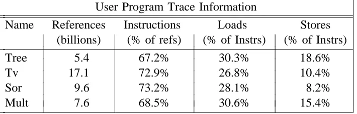
User Program Trace Information _i

iiiiiiiiiiiiiiiiiiiiiiiiiiiiiiiiiiiiiiiiiiiiiiiiiiiiiiiiiii iiiiiiiiiiiiiiiiiiiiiiiiiiiiiiiiiiiiiiiiiiiiiiiiiiiiiiiiii

Name References Instructions Loads Stores )

i_{iiiiiiiiiiiiiiiiiiiiiiiiiiiiiiiiiiiiiiiiiiiiiiiiiiiiiiiiii}(billions) (% of refs) (% of Instrs) (% of Instrs

T

Tree 5.4 67.2% 30.3% 18.6%

v 17.1 72.9% 26.8% 10.4%

% M

Sor 9.6 73.2% 28.1% 8.2

ult 7.6 68.5% 30.6% 15.4% _i

c c c c c c c c cciiiiiiiiiiiiiiiiiiiiiiiiiiiiiiiiiiiiiiiiiiiiiiiiiiiiiiiiiicc c c c c c cc c c c c c cc c c c c c cc c c c c c cc c c c c c c c c

Figure 5: User trace characteristics

Figure 4 contains the characteristics of the example traces. Not surprisingly, the number of instructions as a percent of memory references is higher than in CISC programs. The average percent of references that are instructions is 70.5%, whereas the average value for traces ex-amined in [6] was 53.3%. All of the programs had been compiled with all available optimization including global register allocation [17].

7.3. CPI as a Measure of Cache Behavior

The most common measure of cache performance is the miss ratio, the fraction of requests that are not satisfied by a cache. Though the miss ratio is useful for comparing individual caches, it does not give a clear picture of the effect of a cache’s performance on the performance of the machine as a whole, or of the relative importance of the performance of each cache in a multi-cache system. For example, one cache may have a much higher miss ratio than another, but be used much less frequently and result in less overall performance degradation than the first.

A better measure of performance in a multi-cache system is CPI, the average cycles per

instruction. CPI accounts for variations in the number of references to the different caches and

differences in the costs of misses to the caches, and can be broken down into the components contributed by each part of the memory hierarchy. We are concerned only with memory delays and ignore all other forms of pipeline stalls, assuming one instruction is issued per cycle. There-fore, for our base machine the total CPI over some execution interval is:

where CPI_cache-typeis the contribution of a cache and CPI_wtbufferis the contribution of the write buffer.

If for each cache,

m_cache-type= number of misses during the interval

c_cache-type= cost in cycles of a miss

i = the number of instructions in the interval

then

CPI_cache−type= (m_cache−type×c_cache−type) / i

The goal is to minimize the total CPI.

Admittedly, CPI is an architecturally dependent measure, but machine designers are most of-ten interested in the performance of a specific architecture rather than cache performance in a vacuum. CPI_total tells much more about the performance of our base architecture than do the miss ratios of the individual caches.

For example, the top graph in Figure 6 shows the miss ratios for the three caches during a 3 billion instruction segment of a run of the Mult set of programs. The bottom graph shows the total CPI and CPI contribution of each cache for the same run. While the miss ratio for the data cache usually exceeds that of the instruction and second level caches, its actual contribution to the total CPI is much smaller than that of the instruction or second level caches. The CPI graph also shows that the second level cache often contributes nearly twice as much to the overall performance degradation as do either the instruction or data caches.

In the rest of this paper, we will present trace results in terms of two different measures of

CPI, the interval CPI and the cumulative CPI. The interval CPI is measured at regular intervals

over the course of a trace and simulation run and at each point is the average for the previous interval. The cumulative CPI is the CPI averaged over the entire preceding portion of a run.

7.4. Long Traces are Nice and Necessary

Some of the earliest data collected validated our belief that long traces were necessary to un-derstand the behavior of large caches. Each point in Figure 6 represents an average over 100 million instructions, or approximately 150 million memory references. Most existing traces are less than 10 million references long. Each point in Figure 6 is ten times that. The variation in the CPI_totalover the length of the trace makes clear the necessity of long traces.

5 5.5 6 6.5 7 7.5 8 Instructions Executed (Billions)

0 0.1

0.02 0.04 0.06 0.08

Interval Miss Ratio

instr data level 2

5 5.5 6 6.5 7 7.5 8

Instructions Executed (Billions) 0

4

1 2 3

Interval CPI

instr data level 2 total

Figure 6: Interval miss ratios (top) and interval CPIs (bottom) for Mult

In the above examples, the CPIs and miss ratios were measured at intervals of 100 million instructions. The instruction and data caches are both 4K bytes consisting of 256 4-word lines. The second level cache is 16M bytes made up of 4096 32-word lines. All three are direct-mapped.

1060 1080 1100 1120 1140 Instructions Executed / 10M

0 7

1 2 3 4 5 6

CPI for Prev 10M Instrs

instr data level 2 total

1140 1160 1180 1200 1220

Instructions Executed / 10M

0 7

1 2 3 4 5 6

10 million instructions. The total length of most available traces.

Figure 7: Interval CPIs for TV in two parts

lows in the graph of CPI_instare loops that execute small sections of code and go through large volumes of data.

.02 .04 .06

.0 .08 .10

miss ratio

Tree

short trace long trace

direct

2-way 4-way

.02 .04 .06

.0 .08 .10

2-way 4-way

direct

SOR

miss ratio

*

*

4K 16K 64K 256K 1M

1M 256K

64K 16K

4K

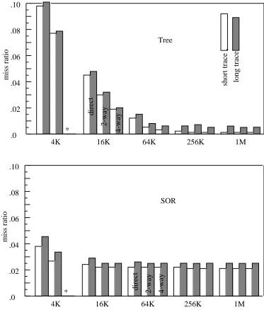
Figure 8: Miss ratios for short (500K refs) and long (150M refs) traces

Data was collected for 5 cache sizes, 4K to 1M. The data are for single level mixed instruction and data caches. * Note that there is no data for the 4K byte cache with 4-way associativity.

problems since Tycho accounts for them. The miss ratio will not always be lower for long traces. The difference depends on where in a long trace the short trace is chosen. Were we to run the same experiment with TV, choosing an early part of the run for the short trace, the miss ratio would undoubtedly go up. In general the results show that the differences are greater, and so long traces are more essential for large caches and higher degrees of associativity.

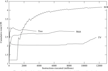
We have shown that very long traces give a great deal of information about a program’s be-havior and that using traces that are too short can lead to erroneous performance estimation. We have not yet dealt with the question of how long a trace must be to get valid performance data. How long is long enough? Unfortunately, that depends on the application or set of applications running. The graphs in Figure 9 show this clearly. Tree terminates before it stabilizes. SOR gradually stabilizes after 10 billion references. TV appears to stabilize early and then takes a jump after 10 billion references. Only Mult seems to stabilize reasonably well, and even so takes at least 1 billion references to do so. It appears that even to have the cache warm up one needs a trace of 500 million references!

0 2000 4000 6000 8000 10000 12000

Instructions executed (millions) 1

4.5

1.5 2 2.5 3 3.5 4

Cumulative total CPI

TV SOR

Tree _Mult

Figure 9: Cumulative CPI_totalfor the four examples with a 512K second level cache.

In each case, both first level caches had 4K bytes with 16 byte lines. The second level cache had 512K bytes in 128 byte lines. All were direct-mapped.

7.5. Address Mapping to the Second Level Cache

which is the same for virtual and physical addresses, can be used to identify the appropriate cache line. A process id field associated with each cache line determines whether the contents of the cache line is from the correct address space. In this case, misses will be identical to those occurring in a physical cache where the pid field is replaced by a physical page number field. When the cache is very much larger than the page size, as will almost certainly be the case for the second level cache, the page offset maps to only a tiny proportion of the cache.

If an address’s offset relative to the cache size is used as a mapping, sequential virtual ad-dresses will map sequentially into the cache, wrapping around only when they are larger than the cache size. Since the cache may be larger than the address space of many programs, all of those programs will conflict in those portions of the cache associated with commonly used virtual ad-dresses. Even for large programs, instruction addresses, which map into the low addresses, will conflict.

A similar mapping based on physical addresses should provide better distribution throughout the cache. Physical addresses, which are sequential only within pages, will be scattered through-out the cache in page-sized chunks, assuming that the physical memory is very much larger than the second level cache. Their distribution in the cache will depend on the memory management algorithm. Unfortunately, using the actual physical address from the Titan in our simulations is unrealistic. Not only is the Titan’s physical memory too small, but the physical addresses for user code correspond to the expanded trace code rather than the unexpanded real code.

Since the cache is so large, one should be able to spread out references from different processes, eliminating interprocess conflicts, and assuring that much of a process’s working set remains in the cache after process switches. The two-level cache simulations performed by Panama use a simple pid hashing algorithm to distribute mappings in the cache. The goal of pid hashing is to reduce cache conflicts due to the "bunching" of references to particular areas in the address space. The pid is exclusive-ORed with the part of the address that indexes into the sets of the cache. Thus, the same virtual address from different address spaces will map into dif-ferent areas of the cache, reducing conflicts. This method may be viewed as a possible im-plementation for a virtually addressed cache or as an approximation of the distribution naturally provided by physical addressing.

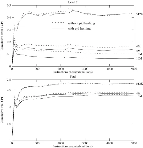
The graphs in Figure 10 compare the cumulative CPIs for three sizes of second level cache when pid hashing is used (dotted lines) and when the address modulo the cache size is used (solid lines). The upper graph shows CPI_level2. The lower graph shows CPI_total. Pid hashing effectively reduces CPI_level2 only when the cache is quite large. Even in the best case, when it reduces the second level contribution for a 16 megabyte cache by about 30% it has less than 1% effect on the CPI_total. As cache size increases, pid hashing more effectively reduces the miss rate and thus the CPI_level2. On the other hand, as cache size increases, the miss rate and

0 1000 2000 3000 4000 5000 Instructions executed (millions)

0 0.5

0.1 0.2 0.3 0.4

Cumulative level 2 CPI

Level 2

512K

4M 4M

16M 16M

without pid hashing

with pid hashing

0 1000 2000 3000 4000 5000

Instructions executed (millions) 1

2.8

1.5 2 2.5

Cumulative total CPI

Total

512K

4M 16M

Figure 10: Effectiveness of pid hashing for 512K, 4M, and 16M second level caches

Cumulative CPIs for 5 billion instruction runs of Mult with pid hashing (solid lines) and without pid hashing (dotted lines). The upper graph shows only the CPI_level2. The lower graph shows the CPI_total.

7.6. Multiple Process Traces

programs represent differences that will occur on a real machine. On the other hand, variations between runs may make it difficult to precisely understand the significance of variations due to cache modifications.

0 500 1000 1500 2000 2500 3000

Instructions executed (millions) 1

2.6

1.5 2 2.5

Cumulative total CPI

4M 1M

16M

Figure 11: Variations in multiprocess runs

For all eight runs the first level caches were 4K bytes with 16 byte lines. The second level caches were 1M and 4M bytes with 128 byte lines and 16M with 256 byte lines.

Figure 11 shows the cumulative CPI_totalfor repeated runs of Mult at three second level cache sizes. The variations between same sized runs are quite small, usually less than 1%. In all of our experiments, variations in cache characteristics caused changes in the CPI results that were ei-ther significantly and consistently greater than 1% or the fact that they were smaller was by itself a useful result. In cases were more specific detailed distinctions between similar results are needed, we will modify the cache analysis program to simulate multiple caches at the same time. The need for this has not yet risen.

7.7. Second Level Cache Size

Next, we present the results of varying only the size of the second level cache. We did not simulate the case without a second level cache but can easily argue that its performance would be unacceptable. Assuming miss ratios of 5% for the data and instruction caches, a 200 cycle cost for each miss, and that the data cache is used 40% as often as the instruction cache, the

8.5 9 9.5 10 10.5 11 11.5 0

4

1 2

3 TV

512K 4M

16M

3 3.5 4 4.5 5 5.5 6

0 5

1 2 3

4 SOR 512K

4M

16M

0.5 1 1.5 2 2.5 3 3.5

0 1.4

0.2 0.4 0.6 0.8 1 1.2

Interval Level2 CPI Tree 512K

4M 16M

2 2.5 3 3.5 4 4.5 5

Instructions Executed (Billions) 0

1

0.2 0.4 0.6

0.8 Mult

512K 4M 16M

Figure 12: Interval CPI_level2for three second level cache sizes

Figure 12 shows the CPI_level2 for three sizes of the second level cache: 512K, 4M, and 16M. Except during the early part of the TV run, there is a dramatic reduction in CPI_level2 when the cache size is increased to 4M but a considerably smaller improvement resulting from the jump to 16M.

Interval CPI gives a good picture of the different behaviors of the programs, however, the cumulative CPIs shown in Figure 13 shows the effect of cache size increases on long run average system performance. SOR, with its periodic behavior, is the only program that greatly benefits from an increase to 16M. This is most likely because it actually references a large part of its large address space. We can conclude from these examples that most of the programs we have chosen do not have large working sets. Mult is the most realistic of the examples, however, its usefulness is limited by the relatively small size of each of the individual programs it runs. There is definitely a need to put together much larger multiprocessing workloads.

We can get a bit more insight into the existing data by dividing level 2 cache misses into three categories defined by Hill [6]: compulsory, capacity, and conflict. Compulsory misses happen the first time an address is referenced and and occur regardless of the size of the cache. Our simulator computes the compulsory, fully associative, and direct-mapped miss ratios. The capacity miss ratio is the difference between the fully associative miss ratio and the compulsory miss ratio. The conflict miss ratio is the difference between the direct-mapped miss ratio and the associative miss ratio. From these values we have computed the percent of misses in each cate-gory for the Mult runs for each cache size shown in Figure 14.

Capacity misses are due to fixed cache size. The percent of capacity misses decreases markedly when the cache size in increased to 4M bytes, but very little more as the result of the increase to 16M. Conflict misses result from too many mappings of addresses to the same cache lines. The percent of conflict misses increases slightly from 512K to 4M, but decreases substan-tially when the cache size is increased to 16M. Thus, beyond 4M, increases in size primarily allow interfering blocks to be spread out more effectively. This corresponds to the increased effectiveness of pid hashing to reduce the miss rate for a 16M cache.

7.8. Direct-Mapped vs Associative Second Level Caches

In this section, we examine the effects of associativity in large second level caches. Increasing associativity can decrease the miss ratio of a cache, but it may have limited effect or even an adverse effect on the performance of the system as a whole [5]. If the cache is very large, having a low miss ratio in the direct-mapped case, then reducing the miss ratio can only have a small effect on overall performance, even if associativity comes with no cost. It is more likely that for large caches, the cost of implementing associativity outweighs its benefits. The positive effects of associativity are related to the cache’s miss ratio, but the negative effects in added cost are related to the total number of references to the cache. Though increased associativity may decrease the number of misses and thus the total cost of misses, it makes every reference to a cache more expensive.

0 2000 4000 6000 8000 10000 12000 1.2 2.5 1.4 1.6 1.8 2 2.2 2.4 TV 512K 4M 16M

0 2000 4000 6000 8000 10000 12000

1 4.5 1.5 2 2.5 3 3.5 4 SOR 512K 4M 16M

0 2000 4000 6000 8000 10000 12000

2 3.2 2.2 2.4 2.6 2.8 3

Cumulative total CPI Tree 512K

4M 16M

0 2000 4000 6000 8000 10000 12000

Instructions executed (millions) 1.5 3 1.6 1.8 2 2.2 2.4 2.6 2.8 Mult 512K 4M 16M

Figure 13: Cumulative CPI_totalfor three second level cache sizes

LONGADDRESSTRACESfROMRISCMACHINES

iiiiiiiiiiiiiiiiiiiiiiiiiiiiiiiiiiiiiiiiiii

Categories of level 2 misses _i

iiiiiiiiiiiiiiiiiiiiiiiiiiiiiiiiiiiiiiiiiii iiiiiiiiiiiiiiiiiiiiiiiiiiiiiiiiiiiiiiiiii

Cache Size conflict capacity compulsory

i_{iiiiiiiiiiiiiiiiiiiiiiiiiiiiiiiiiiiiiiiiii}(%) (%) (%)

512K 40.4 57.6 2.0

4M 41.5 47.3 11.2

9

i_{iiiiiiiiiiiiiiiiiiiiiiiiiiiiiiiiiiiiiiiiii}16M 32.0 45.1 22.

cc c c c c c c c c c c c c c c c c c c c cc c c c c c c c

Figure 14: Compulsory, capacity, and conflict misses

shows the cumulative CPI_totalin the direct-mapped and associative cases for Mult runs with four second level cache sizes. The results show that even in the most optimistic case, associativity is minimally effective for large caches (4M and 16M) but may be useful for 1M or 512K caches.

0 2000 4000 6000 8000 10000

Instructions executed (millions) 1 2.9 1.5 2 2.5 Cumulative CPI 512K 1M 4M 16M

Figure 15: CPI_totalfor direct mapped and fully associative cases

Cumulative CPI_total for Mult for direct-mapped (solid) and fully associative (dotted) for four cache sizes.

Using subscripts a and d to indicate associative and direct-mapped, respectively,

CPI = CPI +_{a d} ∆CPI

= CPI + R_{d 1}⋅( A_a−A )_d

where A and A are the average cost per reference to the second level cache, and R is the first_{a d 1} level miss ratio (combined for data and instruction caches).

Letting

∆A = A_a−A_d

and

h = cost of a hit in the associative cache_a

h = cost of a hit in the direct-mapped cache_d

m = cost of a second level cache miss (same direct-mapped and associative)

R = miss ratio for a second level associative cache_a

R = miss ratio for a second level direct-mapped_d

then,

∆A = h_a⋅R + m_a ⋅(1−R )_a −(h_d⋅R + m_d ⋅(1−R ) )_d

= h_a⋅R_a−h_d⋅R + m_d ⋅(R_d−R )_a

Expressing this as a function of h and the ratio_d

h_d

k =

h_a

we get

1

∆A = h_d⋅( ⋅R_a−R ) + m_d ⋅(R_d−R )_a

k

and

1

CPI = CPI + R_{a d 1}⋅(h_d⋅( R_a−R ) + m_d ⋅(R_d−R ))_a

k

Since the miss ratios do not depend on reference costs, we use the miss ratios and CPI from_d our simulations to plot the CPI versus k for the values of h and m used in the simulation. he_{a d} results are shown in Figure 16. The horizontal lines represent CPI , the direct-mapped value, for_d each cache size. The corresponding sloping lines represent CPI , the fully associative value, for_a various values of k. The diamonds note the crossover points at which the CPI is the same in the associative and direct-mapped cases. The distance between the points at which corresponding horizontal and sloping lines intersect the vertical at k = 1 is the maximum gain to be expected from associativity, assuming that full associativity provides an upper bound on that gain.

0.8 0.9 1 1.1 1.2 1.3 1.4 k 2 3 2.2 2.4 2.6 2.8 CPI Mult

0.8 0.9 1 1.1 1.2 1.3 1.4

k 2 3 2.2 2.4 2.6 2.8 CPI Tree

0.8 0.9 1 1.1 1.2 1.3 1.4

k 2 3 2.2 2.4 2.6 2.8 CPI TV

0.8 0.9 1 1.1 1.2 1.3 1.4

k 1.6 4.2 1.8 2 2.2 2.4 2.6 2.8 3 3.2 3.4 3.6 3.8 4 CPI SOR

512K 4M 16M

Figure 16: CPIs for fully associative caches as function of implementation cost

detailed simulations using realistic costs and degrees of associativity. In these three case, as expected, all diamonds are to the right of k = 1. That is, performance improves with full sociativity. Yet, the intersection in the 16M case is very close to k = 1 implying that as-sociativity would have to be nearly free to get even a small gain. On the other hand, for a cache size of 512K, if associativity could be implemented for a cost per reference of 10% or less, all three of the benchmarks would see some improvement in performance.

7.9. Line Size in First and Second Level Caches

We have done some preliminary experiments with changes in line size in both the first and second level caches. The solid lines in Figure 17 show the effects of doubling and then quad-rupling the line size for both the first level caches. These runs were made with a 512K second level cache, but the reduction in first level contributions are independent of the second level size. Most of the improvement is due to the deceased contribution of the instruction cache. CPI_data stayed nearly constant. The improvement in memory system performance as the result going from 16 to 32 byte lines without changing the capacity of the cache is about the same as that of increasing the size of the second level cache 8 times. The dotted line shows CPI_totalfor a 4M second level cache and 16byte lines in the first level cache. Unfortunately, doubling the line size of an on chip cache is not a trivial matter. It may be that using some form of prefetch will be less difficult and nearly as effective.

0 500 1000 1500 2000 2500

Instructions executed (millions) 1

3

1.5 2 2.5

Cumulative total CPI

16 byte/512K

64 byte/512K 32 byte/512K 16byte/4M

Figure 17: Three lines sizes for the first level caches

Solid lines show variations in the line size of the first level caches with a second level cache size of 512K. The dotted line is from a run with a 4M second level cache and 16 byte lines in the first level cache.

Doubling the length of lines in the second level cache from 128 bytes to 256 bytes made al-most no difference in performance as shown in Figure 18. The difference is within the 1% varia-tion found between runs of Mult with constant cache characteristics. This is the case even though the cost of retrieving the two line sizes was identical in the tow runs. Apparently, there is too much conflict for long line sizes to be beneficial.

7.10. Write Buffer Contributions

0 500 1000 1500 2000 2500 Instructions executed (millions)

1 3

1.5 2 2.5

Cumulative total CPI

128 byte/16M 256 byte/16M

Figure 18: Two line sizes a 16M second level cache

Closer examination showed the reason to be the the sensitivity of write buffer performance to both the proportion and distribution of writes in the instructions executed. A write buffer entry is retired every six cycles. One would expect it to perform badly if on average more than one in six instructions was a write. In addition, bunching of the writes, rather than even distribution com-pounds the problem.

The graphs in Figures 19 and 20 show the clear relationship between the proportion of writes in a program and the write buffer performance. Whenever the percent of writes goes about one in six or 17%, the CPI_wtbuffertakes a proportionally greater jump. The change in CPI_wtbuffer in the 2000M-5000M instruction range in the Mult graph of Figure 19 is most likely the result of the smaller run of Tree executed as part of the Mult set of programs. This lead us to look more closely at the difference between the compiled Scheme code for Tree and that for the other programs.

To determine this correlation more precisely, we plotted the CPI_wtbuffer against percent of in-structions that are writes. The graphs in Figures 21 and 22 show both the effect of the proportion of writes and the distribution of writes. Although our simulations do not measure the distribu-tion of writes, some trends are apparent from the graphs. The tendency of CPI_wtbuffer values associated with a percent of writes to be very close together indicates a consistent degree of bunching. Variations in the distribution of writes shows up as a spread of values for each per-centage.