APPLICATION OF MULTIOBJECTIVE TECHNIQUE TO
MULTI-DISCIPLINARY OPTIMAL POWER FLOW PROBLEM
USING REFINED FORAGING ALGORITHMS
1
S.JAGANATHAN
,
2 S.PALANISWAMI1Asstt Prof., Department of Electrical Engineering, RVS College of Engineering and Technology, Coimbatore, Tamilnadu, India
2 Principal, Government College of Engineering, Bargur, Tamilnadu, India. E-mail: [email protected], [email protected]
ABSTRACT
TheOptimal Power Flow (OPF) is important problem in electric power systems and OPF is a static, non – linear optimization problem of determining the optimal settings of control variables for minimization the cost of generation including sine components, piecewise quadratic cost curve, transmission losses, voltage profile optimization and power flow deviations are proposed in this paper. The OPF problem is not only comprised of cost of generation and includes multidisciplinary comprehensive model. It is an important problem in power systems operation due to operational security considerations and even a small savings per hour translates into large annual saving. A Refined Bacterial Foraging Algorithm [RBFA] is introduced in this paper to solve multi objective optimization problems. The multiobjective is proven and is well in power system problems. The objective of this paper is to introduce RBFA to solve multi disciplinary Optimal Power Flow [MDOPF] based on multi-objective optimization. The new multiobjective BFA is presented for the solution of the comprehensive model for MDOPF. The algorithm is then demonstrated on IEEE 30 bus system and test results provided on the standard system reported in the literature clearly indicates that this method is efficient. The RBFA is motivated by the foraging behavior of the E. coli bacteria and the biological aspects of the bacterial foraging strategies and is well in multi disciplinary high dimensional problems and multiple objective optimization problems. The solution of the MDOPF problem, with a simultaneous and adequate consideration of all its facets with reasonable computing time, is still to be achieved.
Keywords: Refined Bacterial Foraging Algorithm, Multi-Disciplinary Optimal Power Flow, Quadratic Curve With Sine Components, Piecewise Quadratic Curve, Voltage Profile Optimization And Active Power Losses.
1. INTRODUCTION
The multi disciplinary optimal power flow (OPF) problems have to be solved to operate the power system in optimal and secure region; this problem is related to concern with quality and reliability of power supply and also economy and security of the power systems. It is an essential function in power system planning and operation, because the solution of OPF [5] is found to solve the conventional power flow equations [5], [8], [9] while at the same time minimizing all objectives and meeting the requirements of power system. The resulting optimization problem has nonlinear constraints from the power flow nodal equations and simple bound constraints on the variables from the load bus voltage magnitudes. The purpose of an Optimal Power Flow function is to schedule the power system controls to optimize an objective function
while satisfying a set of nonlinear equality and inequality constraints. The equality constraints are the conventional power flow equations; the inequality constraints are the limits on the control and operating variables of the system, main concern towards power system is to produce better results for power flow optimization problem with enhanced stability and economy [18], [16].
Mathematically the OPF can be formulated as a constrained nonlinear optimization problem. Practical, constrained active and reactive OPF problems have complicated analytical, non-static and partially discrete formulations. At the same time, however, most OPF development efforts have centered on the mathematical optimization of simple classical OPF formulations, [20], [21], [22] expressed in smooth nonlinear programming form. However, the Optimal Power Flow has had a long history in its development. Thirty years ago, Carpentier introduced a generalized, nonlinear programming formulation of the economic dispatch problem including voltage and other operating constraints. This formulation was later named as the Optimal Power Flow problem [11]. Historically different solution approaches have been developed to solve these different classes of the OPF problem. The OPF problem has a long time to become a successful algorithm [20] that could be applied in everyday use. Current interest is the OPF centers around its ability to solve for the Optimal Solution that takes account of the security of the power system.
GA, invented by Holland in the early 1970s, is a stochastic global search method that mimics the metaphor of natural biological evaluation. GA operates on a population of candidate solutions encoded to finite bit string called chromosome. In order to obtain optimality, each chromosome exchanges information’s by using operators borrowed from natural genetic produce the better solution [7]. The GA uses only objective function information, not derivative or other auxiliary knowledge. Therefore, GA can deal with the non-smooth, non-continuous and non-differentiable functions, which actually exist in a practical optimization problem. On the other hand, [8] EP is also a global search method starting from a population of candidate solutions, and finds solution in parallel using evaluation process. Both GA and EP can provide a near global solution. However, the encoding the decoding schemes essential in the GA approach are not needed in OPF problem. Therefore, EP is faster in speed than GA in this case [11].The social and foraging behavior algorithms are recent developments in searching algorithms and it’s widely used to solve optimization problems [5], [6] .The hybrid technique algorithm is also very useful for the solution of the optimization problems, mainly hybrid algorithms tensed to produce better results than individual analysis [15]. Various algorithms have been proposed to solve the Optimal Power
Flow problem and all above discussed algorithms are can be deal only Single Objective Optimization problems and it provides unique optimal solutions. However, there are many situations where decisions have multiple objectives in these situations to optimize a group of conflicting objectives Multi Objective Optimization (MOP) is used [24], [3].
The recent development of multi-objective optimization technique based on genetic algorithm gives the ability to treat objectives of optimization problems independently. The simultaneous optimization is required, when number of objectives to be optimized. In recent years, multiobjective problems have arose in many engineering applications. Many algorithms involved in multiobjective solutions, but only few algorithms are successful [1], [2]. In this paper, the application of foraging behavior based algorithms is used to solve MDOPF problem and RBFA is proposed. The proposed method can provide a good solution even the problem has many local optimum solutions at the beginning. In order to show the effectiveness of the proposed method over an existing technique, this method is capable of determining the global optimum solution to the OPF for a range of constraints and objective functions. The algorithm is not sensitive to starting points and is capable of handling non-convex generator cost curves. Computational implementation results involving IEEE standard test systems are given to demonstrate the validity of this method, and results are comparable with technique.
2. PROBLEM FORMULATION
Optimal Power Flow: Generally the optimal
power flow problem can be expressed as follows:
Objective function
Minimize f x
( )
Subject to the constraints
( )
0 1, 2....,g x i m n
i = =
( )
0 1, 2....,h xi = i= n (1)
Where: x∈Rn is the vector of the state
variables; f x
( )
is real power loss in transmission;( )
0i
( )
0i
h x ≤ is the set of limits on state variables and power system functional constraints [18], [23] [6].
The state variable vector X represents the voltage magnitude, real and reactive power, phase angles, LTC’s taps and reactive power compensator. The objective function, f x
( )
, canassume different forms, for example, the active power losses in transmission, the active power cost of dispatchable generators, non-smooth cost functions and quadratic functions. The equality constraints gi
( )
x =0represent the power flowequation. The inequality constraints h xi
( )
≤0represent the functional constraints of the power flow, i.e., limits of active and reactive power flows in the transmission lines and transformers, limits of reactive power injections for reactive control buses and active power injections for reactive control buses and active power injection for the slack bus. This is a typical nonlinear and nonconvex problem.
f - is the objective function to be minimized, g - is the equality constraint. h-is the system operating constraints.
MDOPF Problem Formulation: The MDOPF
formulation consists of the objective function and equality constraints and inequality constraints. While formulating this type of important power system problem, our primary concern is in the identification of variables during the process. In order to handle these variables in the MDOPF problem efficiently, it is convenient to separate them into three categories: controls, state, and constraints. The control variables correspond to quantities that can be arbitrarily manipulated, within their limits, in order to minimize the cost both smooth and non-smooth functions. These include generator real and reactive power outputs, transformer tap settings, and reactive power compensator, bus voltage levels and voltage profile optimization.
Objective Function: The objective functions of
OPF are all usually minimization case. In some
cases, such as power transfers, it may be maximized. Here, we shall choose the objective function as f .The MDOPF objectives are given in this section guarantee and all objectives should met the power flow constraints
Cost function: To minimize the
)
2 1f ai b Pi gi c Pi gi i Ng
= ∑ + +
∈ (2)
Where
a
i,b
i andc
iare the generator costcoefficients at ith generation
Real Power Loss: This objective is to minimize
the real power loss in transmission lines that can be expressed as:
( )
2 2
Vi V – 2V V cos j i j i– j 1
L Nl
P Gk
k δ δ
=∑ = +
(3)
Where Nl is the number of transmission lines; Gk is the conductance of the kth line; Vi<δi and Vj<δj are the voltages at the end buses i and j of the kth line respectively.
Active Power Losses:P =Pgi- Pload ≥ 0
(
2 2)
2 cos
gi E
l l ij i j i j ij
k N K n
f P g v v v v θ
= =
=
∑
=∑
+ −(4)
Where P is the total transmission active losses of the power system in MW; Pgi is the total active power generated in MW, Ploss the total transmission losses in the network to be calculated in MW and Pload is the total load of the system in MW.
Voltage profile optimization: Bus voltage is
one of the most important security and service quality indices. Considering only cost-based objectives in OPF problem may result in a feasible solution that has unattractive voltage profile. In this case, a twofold objective function is considered in order to minimize the fuel cost and improve voltage profile
(
)
2(
)
2(
)
2lim lim lim
1.0
2 1 1
1 1 1
NG NL NL
f f w v P P V V Q Qg
i i P g g v i i Q gi i
i i NL i i
λ λ λ
= ∑ + ∑ − + − + ∑ − + ∑ −
= ∈ = =
(5)
by minimizing the load bus voltage deviations from 1.0 per unit.
The objective function of MDOPF problem can be expressed as
Minimize F= f P P V VmL d (6)
Subject equality and in-equality constraints are given below sections.
Quadratic Cost Curve: Other objective function
2 F = ai +b Pi gi +c Pi gi (7)
Where ai,bi and ci are the cost coefficients of the ith generator. This technique was tested for several initial solutions and the different initial solutions are generated by changing the value of bacteria seed the variations of the objective function with different initialization are considered for test cases. It is clear that the technique converges to the optimal solution regardless of the initial one.
Quadratic cost curve with sine components: Approximating the cost curves by smooth quadratic functions results in some inaccuracy due to neglecting the ripples produced by the valve point loading. In this case, a sine component is superimposed to the cost curves of the generators buses to reflect the valve point loading effects as
( )
2
sin min
F=ai+b Pi gi+c Pi gi+di eiPgi − Pgi
(8)
Where
i
= No. of generator busesai, bi, ci, di and ei are the cost coefficients of the ith generator. The cost curves of the other generators are the same as in case quadratic cost curve.
Piecewise quadratic cost curve: In this study,
units 1 and 2 cost curves were replaced by piecewise quadratic curves summarized to model different fuels or valve point loading effects. In order to allow more precise control over units with discontinuities in cost curves, the unit with the simplest type of cost curve and largest capacity was selected to be the slack node. The generation Piecewise Quadratic Cost Curve function is
2
F=ai+b Pi gi+c Pi gi (9)
Where
ai, bi and ci are the cost coefficients of the ith generator.
Constraints
Equality Constraints
Subject to the power flow equations
)
(
)
Pi Ei G Eij j B Fij j Fi G Fij j B Eij j
j N j N
= ∑ − + ∑ −
= =
1, 2, 3,..., ,
i= N i ≠ s
)
)
Q E G E B F F G F B E
i i ij j ij j i ij j ij j
j N j N
pq pq
= ∑ − + ∑ −
= =
1, 2, 3,...,
i= N pq (10)
Where, N is the No. of buses and Npq is the No. of Load buses.
In-Equality Constraints
Generation Constraints: Generator voltages, real
power outputs and reactive power outputs are restricted by the lower and upper limits.
min max ;
P P P i N
gi ≤ gi ≤ gi ∈ G
min max;
Qgi ≤ Qgi ≤ Qgi i ∈ NG
min max ;
Vgi ≤ Vgi ≤ Vgi i ∈ NG (11)
Where, N is the No. of buses, Pgi is real power in the ith bus, Qgi isreactive power in the ith bus, Vgi is real power in the ith bus.
Transformer Constraints: Transformer tap settings
are restricted by the lower and upper limits.
min max;
Ti Ti Ti i N
T
≤ ≤ ∈ (12)
Where, NT is the No. of regulating or tap-setting transformers.
Reactive Power Compensators: Reactive power
compensators are restricted by the lower and upper limits.
min max;
Q Q Q i Nc
ci ≤ ci ≤ ci ∈ (13)
Where, Nc is the No. of Reactive power compensating buses, Qci is reactive power compensation with help of compensating deices.
It is worth mentioning that the control variables are self-constrained. The hard inequalities of Pgi and Qgi can be incorporated in the objective function. The power equations are used as equality constraintsand the inequality constraints are active and reactive power generation restrictions, transformer tap-setting restrictions, reactive power compensators and apparent power flow restrictions in branches and bus voltage restrictions.
Solution of optimal power flow: MDOPF is an
savings per hour translates into large annual savings) Hence lot of research has been directed towards achieving better solutions of this problem, subsequently we need suitable method to formulate this problem with consider all the objectives and control variables. However, the lack of a suitable method with adequate modeling and solution power limitations on computing power have forced researches to make various simplifications in the above formulation. Therefore the solution of the Multidisciplinary OPF problem, with adequate consideration of all its facets within reasonable computing time, is still to be achieved. The solution methodology be transparent and provides the users with a better visualization of the trade-offs involved in determining an acceptable compromise solution to the problem at hand.
The optimal power flow is a very large and very difficult mathematical programming problem (multidisciplinary problem) and consist one or more associated problems (non-smooth cost function and valve point loading effects). Almost every mathematical programming approach that can be applied to this problem has been attempted and it has taken developers many decades to develop computer codes that will solve the OPF problem reliably. Here, the MDOPF solution is solved with the help of proposed foraging technique. The load flow solution gives the initial solution of MDOPF problem.
Multiobjective Optimization: In many of the real
world problems, involve simultaneous optimization of several objectives functions. These functions are non-commensurable and the functions often-competing objectives. Multiobjective optimization with such objective functions gives a set of optimal solutions, instead of giving one optimal solution. The problem consists of number of objectives to be optimized simultaneously and it is associated with a number of equality and inequality constraints [1], [4].
A general Multiobjective Optimization Problem includes a set of objective functions represented by m and with k restrictions that are the functions of a set of n decision variables. This can be expressed as:
y= F(x) = [F1(x), F2(x)...Fm(x)] (14)
Subject to
E(x) = [E1(x) E2(x) ... Ek(x)] ≤ 0 (15) Where
x= [x1 x2... xn ] ε X, y= [y1 y2... yn ] ε Y
Where x and y are the decision vector and the objective vector.
Load Flow Solution: In order to solve the
multi-objective OPF problem, it is necessary to solve the load flow solution and its existing number of times because, whenever the operating conditions changes the electric power system needs power flow optimization. The RBFA based OPF problem requires, first define the behavior of bacteria initially for initialization of control variables for secure operation and next find the optimal solution with help of Foraging and swimming of bacteria. The algorithm able to find optimal solution subject to load flow convergence and objectives function of cost function both smooth and non-smooth functions. The load flow is solved using a RBFA-based load flow developed using incorporating a Jacobian acceleration stage. In order to keep computation time to a minimum during the optimization, the step length is very much important [1], [6], [7].
The reactive power limits and compensation are the very much important and also major issue in OPF solution but Many OPF solution techniques is failed. While handing these issues it may be produce many violation and distortion during convergence process. The proposed algorithm handles PV buses, PQ buses and these issues, simultaneous optimization and to obtain a load-flow solution. The proposed algorithm handles these issues by the way of simultaneous optimization of all objectives and with help of load-flow solution. Therefore, it is necessary to use the load-flow calculation module in order to make fine adjustments on those optimum values.
Multiobjective and Bacterial Foraging: In this
paper, the modified version of BFA method is combined with a multi-objective approach. The important part in multi-objective bacteria foraging algorithm (MOBFA) is to determine the best global particle for each population and search technique this algorithm is population to population rather than from one individual solution to another makes them very well suited to performing Multiobjective optimization. It is easy to conceive of a population being evolved onto the trade-off surface by a suitably configured BFA. The simultaneous optimization introduced, in order to achieve the solution of multiple objectives problems. In fact, it’s different from single objective optimization solution and adequate change with an appropriate archiving scheme in place [1], [4].
heuristic method, BFA is designed to tackle non-gradient optimization problems and to handle complex and non-differentiable objective functions. Searching the hyperspace is performed through four main operations, namely Chemotaxis, swarming (cell to cell signalling and foraging) reproduction and elimination- dispersal activities.
The chemotaxsis process is performed through swimming and tumbling and this method which is tailored for optimizing difficult numerical functions and based on metaphor of human social interaction and it’s for bacteria gathering to nutrient-rich areas impulsively. Its key concept is that potential solutions are flown through hyperspace and are accelerated towards better or more optimum solutions. Its paradigm can be implemented in simple form of computer codes and is computationally inexpensive in terms of both memory requirements and speed.
3. BACTERIAL FORAGING ALGORITHM
The optimization in BFA comprises the following process: Chemotaxis, swarming, reproduction, elimination and dispersal. Chemotaxis is the activity that bacteria gathering to nutrient-rich areas spontaneously. A Cell-to-cell communication mechanism is established to simulate the biological behavior of bacteria swarming. Reproduction comes from the concept of natural selection and only the bacteria best adapted to their environment tend to survive and transmit their genetic characters to succeeding generations while those less adapted tend to be eliminated. Elimination – dispersal event selects parts of the bacteria to diminish and disperse into random position in the environment, which ensure the diversity of the species [26].
Chemotaxis: This is process achieved through
swimming and tumbling by flagella. Depending upon the rotation of flagella in each bacterium decides it’s pattern, whether it should move in a predefined direction as swimming or altogether in different directions as tumbling in the entire lifetime. The entire lifetime bacteria are set to two mode operation; these modes enable the bacteria to move in the random directions. An E-coli bacterium can move in two different ways alternatively: tumble and run. A tumble is represented by a unit walk with random direction, a unit walk with the same direction as the previous step indicates a run. A chemotactic process is started by one step of tumble and followed by uncertain steps of run, depending on the variation of the environment.
In a tumble, the position of the ith bacterium is updated as:
(
) ( ) ( )
i( j 1, k, l) i j, k, l C i ‹ j
θ + = θ + Φ (16)
Where θI (j,k,l) is the position of the ith bacterium at the jth chemotactic step of the kth reproduction loop in the lth elimination-dispersal event, C(i) is the size of the step taken in the random direction specified by the tumble, <Φ(j) is the angle of the direction which is randomly generated in the range of (0,2π).The fitness value of the ith bacterium at
θi(j,k,l) is represented by ji(j,k,l).If θi(j+1,k,l) the cost is better it means lower then at θi(j,k,l). Now the next step of step size of C(i) in this same direction will be taken and once again, if the step resulted in a position with the better cost the previous step means another step taken. This swim is continued as long as it continuous to reduce the cost and its depending upon maximum number of steps, Ns. The Nc is number of chemotaxis steps.
Swarming: During the process, the E-coli
bacterium produces attraction convergence characteristics and has to desire when anyone bacteria reaches the best position or location, it should attract other bacteria. So, that they converge in that location and this will happen by generation of attraction signal and also in the meantime, each bacterium releases repellent to warn other bacteria to keep a safe distance from. The E-coli bacterium has own in is, a specific sensing, cell to cell signalling, actuation and decision-making mechanism and because of these properties is lead to provide global search . BFA simulates this social behavior by representing the cell to cell signaling
(
) (
)
(
, , , , ,)
(
,(
, ,)
)
1
= ∑ =
i s i i
j j k l j k l jcc j k l
i
θ
θ
θ θ
α
2 exp
1 1
∑ ∑
= s= −d −w p= − i
attract attract m m
i m θ θ
2 exp
1 1
∑ ∑
+ s= h −w p= − i
m m
repellant repellant
i m θ θ
(17) Where
dattract depth of the attractant effect
ωattract measure of the width of the attractant
hrepellant=dattract height of the repellent effect ωrepellant measure of the width of the
P number of parameters to be
optimized
S number of bacteria
Where θi=[θ1,θ2,…….., θp]T is a point optimization domain and it’s the location of the ith bacterium on the P-dimensional optimization domain,θim is the mth component of ith bacterium position, θ={θili=1,2,….,S} represents the position of each member in the population of the S bacteria, θim is the mth component of θ
I
, θim is the mth component of position θt for the tth bacterium, d attract is a quantification of how much attractant is released,
ωattract is a measure of the diffusion rate of the chemical signal, h repellant and ωrepellant are the magnitude and width of the repelling effect respectively, Jicc(θ,θi(j,k,l)) indicates the signals released by the ith bacterium and Jcc(θi, θ) is time-varying function. Jcc(θi,θ) represents the combined attraction and repelling effects received by the ith bacterium.
Reproduction: After Nc chemotactic steps, a
reproduction step is taken. Assume that, Nre is the number of reproduction steps is taken. The final population of bacteria undergoes the reproduction process and here, the least healthy bacteria die and other healthiest bacteria split into two at the same location. All the bacteria are sorted according to their fitness Sr (Sr=S/2, for convenience S is assumed to be a positive even integer) and the step fitness during the life and fitness values for the ith bacterium in the chemotactic loop are accumulated and calculated by:
N Ji(j,k,l) j 1c
∑ =
i N 1
jH Ji(j,k,l)
j 1c+
= ∑ = (18)
Where jiH represents the health of the ith bacterium.
For simplification the number of the bacteria keeps constant in each chemotaxis process. The characters including location and step length of the mother bacterium all reproduced to the children bacteria. Through this selection process the remaining Sr unhealthier bacteria are eliminated and discarded.
Elimination-Dispersal: The process of
chemotaxis and reproduction are not enough for finding global solutions and to improving process of global search ability, the elimination-dispersal event introduced after Nre steps of reproduction. This elimination-dispersal event helps the bacterium avoid
being trapped into local optima and dispersal events may place bacteria near global solutions and also the behavior of bacteria seeks out in favorable environments. The bacteria are eliminated and dispersed to random positions in the optimization domain according to the probability, ped and the number of the event is denoted as Ned.
4. REFINED BACTERIAL FORAGING ALGORITHM
The basic foraging algorithm consists of four steps are Chemotaxis, swarming, reproduction, elimination and dispersal [26]. Chemotaxis is the activity that bacteria gathering to nutrient-rich areas spontaneously. A cell-to-cell communication mechanism is established to simulate the biological behavior of bacteria swarming. Reproduction comes from the concept of natural selection and only the bacteria best adapted to their environment tend to survive and transmit their genetic characters to succeeding generations while those less adapted tend to be eliminated. Elimination –dispersal event selects parts of the bacteria to diminish and disperse into random position in the environment. The proposed method based on foraging behavior of bacteria and some modifications is made through from basic foraging algorithm. The modified algorithm named as Refined Bacterial Foraging Algorithm (RBFA) and RBFA is proposed in this paper. The performance of basic foraging algorithms is well suitable in single objective problems and static environments and step length of the basic BFA is a constant parameter which may guarantee good searching results for small optimization problems. However it is applied to multiple objectives, dynamic environments and high dimensional problems it’s gives poor performance and convergence characteristics also not good and many times it trapped into local optima solutions. The process of search direction and step length is important in multiple objectives and dynamic environments. The proposed approach made some modification in step length; Chemotaxis behavior and adding velocity vector for improve speed of convergence and attaining global solution and also suitable diversity for global search and its improves speed of convergence.
Search direction and Chemotaxis process: The
bacteria step size, unit length, dimension and random direction coordination are much important, a search direction Wid (j) and a step length Lid (j) are calculated separately for each bacteria i, on each dimension d for each time step or tumble-run process or iteration j, Wid (j) =1 means the i-th bacteria goes towards the positive direction of the coordinate axis on the dimension d, its indicates the follow tumble process and consecutive run process. Wid (j) = -1 means the bacteria goes towards the negative direction, its follow again tumble process and Wid (j) =0 means the bacteria stays at the current position; it means the bacteria reaches more nutrient position.
When any one of bacteria finds best position, it should attract other bacteria so that they converge in that location. In this search direction estimation leads to finding the distance of global bacteria from rest of others and the process convergence time minimized. While the distance known, it’s easy to attain the swarming process for new Chemotaxis stage. The current position ith the bacterium, in d dimensional search space and jth tumble-run process is updated
(
)
( )
( )
( )
id id id id
X j+ =1 X j +L j W j (19)
Once the direction and angle is decided by the tumble step, to reach the position it takes several steps (until the position of worst). The rotation angle Ф is related to the number of the dimensions, the number dimensions desired by objectives.
1
round d π φ =
+ (20)
Where, d- search dimension and πis the number of dimensions.
Position updating process: In this process the
step size calculation are initiated with help of position updating process. The basic methodology is adopted in BFA, In order to meet these criteria. The E-coli cells provides attraction signal to each other, so that they swarm or swim together and towards to the best location and swarming pattern based on cell-to-cell communication. But in this process shows slow converge only and in order to improve this process, the velocity factor added with other bacteria so as to reach best bacteria position and this velocity vector added according to other bacteria position. The position updating process mainly focus on best bacteria and each dimension is given by
(
)
(
)
Xid j+ =1 α Xid best−Xid (21)
Where α is a factor to desire the strength of the bacterium’s attraction factor for improving the
strength of the bacterium’s attraction towards to the best position and for faster convergence., Xbest indicates the position of current best global solution updated after each function evaluation, and Xi is the position of the ith bacterium at the jth iteration after the tumble run process.
If a anyone bacteria reaches better position in order to direct the other bacteria to best position, the attraction signal is not enough to reach the best position.
(
)
(
)
Xid j+ =1 α Xid best−Xid +Vj (22)
So, in the process the velocity factor Vj is binding with position updating process and also is pilot to determine the best position according to the previous best positions. Update best bacteria position and add the velocity according to reach the best position, the velocity factor desired by depending upon according to position of best and other bacteria. The velocity factor Vj also gives direction to global best value or its used to identify global best value.
Step length: The basic BFA shows a step size is a
constant parameter and it’s suitable to finding the solution in single and small optimization problems. However, when applied to multiple objective problems and dynamic environmental problems it shows poor performance. The basic BFA with fixed step size is failure in reaching the optimal point for the following reasons. The first case, if step size is very high then the accuracy gets low although the bacterium reaches the locality of optimum point quickly and it moves around the maxima for the remaining chemotactic steps. The second case, if the step size is very small, it takes many chemotactic steps to reach the optimum point and its lead to slow convergence and rate of convergence decreases. Meanwhile to reach the optimal point it takes convergence time and number of iterations increases. So, in order to reach the optimal point, speed of convergence and search ability the controlling of step length is essential. In this paper the proposed RBFA following consideration in determining step length process with help of search dimensions, If deviation is very high then the step size must be increased and if the deviation is small in which case the bacterium is close to the optimum point the step size is to be reduced and also improve the performance the swim walk considered instead of the constant step.
tumble, the location of the ith bacterium is represented by
(
1, ,)
(
, ,) ( ) ( )
L i,id id
X j+ r l =X j r l + j φ j
(23)
Where L i,
( )
j =Lid( )
j Wid( )
jThe J(i,j,k,l) is cost function of corresponding Xid (j,k,l).The fitness value of the ith bacterium at Xid(j,k,l) is represented by jid (j,k,l). In this paper the minimum fitness value jmin is defined as the global optimum.
In a run, consecutive steps of size L(i,j) is the same direction as the tumble is taken, in condition Xid (j+1,k,l) the cost function J (i,j+1, k,l) is better (lower) than J(i,j,k,l). In this condition, the fitness value of the ith bacterium in the rth step of the run Ns indicates the maximum number of steps in a run and also r is smaller than Ns. This swimming operation is repeated as long as a lower cost is obtained until a maximum preset number of steps, Ns, is reached.
In BFA the step length L is a constant and it ensures accuracy and speed of the search. The size of the step length is dynamically adjusted in the reproduction and elimination-dispersal process, which ensures the bacteria moving towards the global optimum quickly at the beginning, and converging to the global optimum accurately in the end. So the ith bacteria in dth dimension search space the step length controlling vector is given by
( )
{
(
( )
)
}
L id =min L id −µ , n (24)
Where
µ - step length vector, n = constant controlling the decreasing rate of the step length. The value of ‘n’ is desired by according to position updating process and Chemotaxis process.
5. COMPUTATIONAL ALGORITHM AND PSEUDO CODE OF RBFA
The multi disciplinary Optimal Power Flow [MDOPF] based on multi-objective optimization problem is can be solved by using Refined BFA.
Read system data, here the standard IEEE30 bus system data [12] is considered. It contains load data, line data and generator data [12] with cost coefficients.
Randomly initialize the position of each bacterium in the domain, set the position and fitness value of the best bacterium. Initialize the parameters: S, p, Nc, NS, Nre, Nc, Ped, L(i), dattract, wattract, hrepellant and wrepellant
Randomly initialize the position of each bacterium in the domain, set the position and fitness value of the best bacterium as Xidb(j,k,l) and jmin (j, k, l) respectively.
FOR (each bacterium i=1: S)
FOR (chemotactic loop j=1: Nc) FOR (dimensions=1: π)
FOR (reproduction loop k=1: Nre) FOR (elimination-dispersal loop l=1: Ned) Evaluate the cost function J(i,j,k,l)
Let Jlast = J(i,j,k,l) so that a lower cost could be found Calculate Ji (j, k, l) and set it as Jlast;
Tumble:
Search direction identified with help of identification process according to RBFA
For bacterium I, set Ji(j,r) as Jlast. A random vector ∆(i), with each element ∆m(i), m=1,2….. p, a random number in the range [-1,1].
Move:
Move to a random direction
'
∆
∆× ∆
by a unit
walk, the new position is calculated by equation and start another chemotactic step.
Compute J(I,j+1,k,l) and use to compute Jcc (θ, P (j+1,k,l)) then use to find the new J(i,j+1,k,l).
Swim: let m = 0 (counter for swim length) While m< Ns (no climbing down too long)
Let m=m+1
If J(I,j+1,k,l)<Jlast let Jlast = J(I,j+1,k,l) then take
another step in the same direction and compute the new J(I,j+1,k,l).
Swim:
Update Xid(j+1, k, l). Recalculate Ji(j+1, k, l); IF (Jcurrent< Jlast)
WHILE (Jir+1(j+1, k, l)<Jir(j+1, k, l) and r<Ns)
Set Jir (j+1, k, l) as jlast; Run:
Update Xid(j+1, k, l)
Set new Jir+1(j+1, k, l) as Jcurrent; Swim:
END IF
END FOR (bacterium) Calculate Jmin (j+1, k, l) END FOR (chemotaxis) Sum:
Evaluate the sum of the fitness value Jihealth for the ith bacterium.
Sort:
Sort bacteria according to their health Jihealth in ascending order.
Split:
The bacteria with the highest Jihealth values, computed by die while the other Sr with the lowest values split and take the same location of their parents
Eliminate other then health bacteria are to be eliminated.
Update:
Update the step length L (i,j).
END FOR (reproduction)
Disperse:
Disperse certain bacteria to random places in the optimization domain with probability Ped.
Update:
Update the step length L (id)
END FOR (elimination-dispersal)
END
If it’s optimal solution is achieved means, the program will stopped
Computational Procedure:
Step 1: Read system data, here the standard IEEE30 bus system data [12] is considered. It contains load data, line data and generator data ([12] with cost coefficients. Input parameters of system, and specify the lower and upper boundaries of each variable.
Step 2: Initialize the number of bacteria and obtain the step length according foraging behavior.
Step 3: The load flow solution and control variables are initialized.
Step 4: After the load flow Solution, the multi-objective and mutli- disciplinary OPF are solved by using Refined BFA and all objectives are optimized by simultaneous optimization.
Step 5: Get the final optimal solution and quit the program, the above all procedure are clearly described in figure.1
6. RESULTS AND DISCUSSIONS
Figure 1: This figure illustrates the flow chart for computational procedure of proposed algorithm.
Figure 2: The Voltage profile optimization is very much important when tuning the control variables for varying power system operating condition, the proposed technique gives better voltage profile and it’s shown in Fig. 2.
Figure 3:The optimal solution of generation cost is shown in Fig.3.The solution started with higher value but finally reached very mimimum of objectives and its is illustrated in Fig.3 gneration cost ($/hr) Vs number of Iteration.
[image:10.612.324.511.382.522.2]Figure4: The IEEE 30-bus test system is shown in Fig.4. It has six generators at buses 1, 2, 5, 8, 11, and 13 and four transformer with off-nominal tap ratio in lines 6-9, 6-10, 4-12, 27-28.
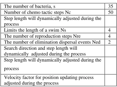
Table1: Simulation Parameters
The number of bacteria, s 35
Number of chemo tactic steps Nc 50
Step length will dynamically adjusted during the process
Limits the length of a swim Ns 4
The number of reproduction steps Nre 4
The number of elimination dispersal events Ned 2
Search direction and step length will dynamically adjusted during the process Step length will dynamically adjusted during the
process
Velocity factor for position updating process adjusted during the process
In this work, the multi-objective optimization technique combined with bacterial foraging algorithms is been used to solve the multi-disciplinary optimal power flow, where it is tested on IEEE 30 bus system. The method described here was implemented in MATLAB7.5 package and simulation results were carried out. The main goal of the experiments was to demonstrate and show the effectiveness of proposed algorithm in various disciplines in optimal power flow problem.
optimization is proposed. The upper and lower limits of tap setting transformers are 0.9 and 1.1 p.u respectively.
The lower limits of voltage magnitude for all buses is 0.95 p.u, the upper limits of voltage magnitude is 1.05 for slack bus and all load busses and upper limits of all other generator buses is 1.1 p.u. The single line diagram of the IEEE 30 bus system is shown in the Fig.2.
The system has six generator buses 1, 2, 5, 8, 11, and 13 and four off-nominal tap ratio in lines 6-9, 6-10, 4-12, and 27-28. The simulation parameters are given in the Table.1.
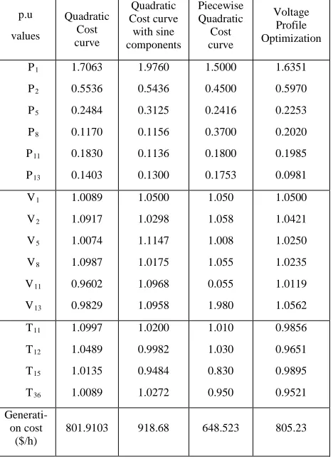
The summary of results of other disciplinary functions like Quadratic Cost curve,Quadratic Cost curve with sine components, Piecewise Quadratic Cost curve and Voltage Profile Optimization are given in Table.2.
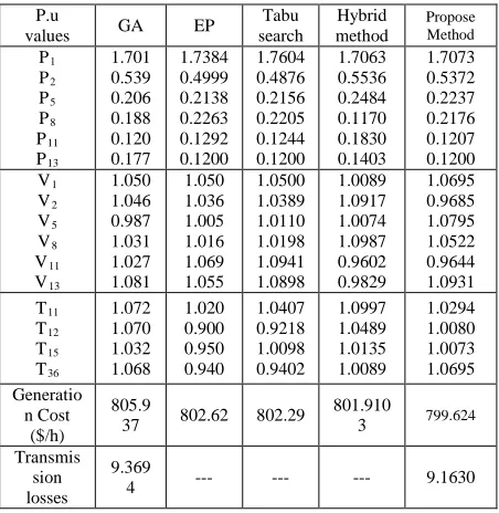
The results of multi-disciplinary optimal power flow for IEEE 30 bus system are given in table.3 and also comparison of results given in same table. The results of proposed algorithm compared with Genetic algorithm (GA), Evolutionary algorithms (EP), Tabu search, and Hybrid algorithm (EP-SQP OPF).
Read System Data’s
Initialization
Load flow solution
RBFA -OPF Control variables analysis
Objective functions Multi-objective Simultaneous optimization
Termination Criteria
Obtain the Global solution
Secure voltage profile and all control variables
End
Start
Fig.1: Flow Chart For Computational Procedure Of Proposed Algorithm
Comparison of Results
Handling of control variables: The proposed
Fig.2: Voltage Profile Optimization
Fig.3: Generation Cost (Y-Axis) Vs No. Of Iterations (X-Axis)
loss is very difficult for different operating conditions, the proposed method is better for handling multi objectives and control variables at any desired operating conditions and it’s proved by reactive power allocation, voltage profile and accordingly transmission loss minimized. Finally the results of proposed method of simultaneous optimization are better for other methods.
Fig.4: Ieee 30 Bus System
Table 2: Summary Of Results Of Simultaneous Optimization Of Multi-Disciplinary And Multi-Objective
OPF For IEEE30 Bus System
p.u
values
Quadratic Cost curve
Quadratic Cost curve
with sine components
Piecewise Quadratic
Cost curve
Voltage Profile Optimization
P1
P2
P5
P8
P11
P13
1.7063
0.5536
0.2484
0.1170
0.1830
0.1403
1.9760
0.5436
0.3125
0.1156
0.1136
0.1300
1.5000
0.4500
0.2416
0.3700
0.1800
0.1753
1.6351
0.5970
0.2253
0.2020
0.1985
0.0981
V1
V2
V5
V8
V11
V13
1.0089
1.0917
1.0074
1.0987
0.9602
0.9829
1.0500
1.0298
1.1147
1.0175
1.0968
1.0958
1.050
1.058
1.008
1.055
0.055
1.980
1.0500
1.0421
1.0250
1.0235
1.0119
1.0562
T11
T12
T15
T36
1.0997
1.0489
1.0135
1.0089
1.0200
0.9982
0.9484
1.0272
1.010
1.030
0.830
0.950
0.9856
0.9651
0.9895
0.9521
Generati-on cost ($/h)
[image:12.612.75.302.324.525.2]Table 3: Summary Of Results Of Multi-Objective OPF For IEEE30 Bus System And Comparison Of Results
P.u
values GA EP
Tabu search Hybrid method Propose Method P1 P2 P5 P8 P11 P13 1.701 0.539 0.206 0.188 0.120 0.177 1.7384 0.4999 0.2138 0.2263 0.1292 0.1200 1.7604 0.4876 0.2156 0.2205 0.1244 0.1200 1.7063 0.5536 0.2484 0.1170 0.1830 0.1403 1.7073 0.5372 0.2237 0.2176 0.1207 0.1200 V1 V2 V5 V8 V11 V13 1.050 1.046 0.987 1.031 1.027 1.081 1.050 1.036 1.005 1.016 1.069 1.055 1.0500 1.0389 1.0110 1.0198 1.0941 1.0898 1.0089 1.0917 1.0074 1.0987 0.9602 0.9829 1.0695 0.9685 1.0795 1.0522 0.9644 1.0931 T11 T12 T15 T36 1.072 1.070 1.032 1.068 1.020 0.900 0.950 0.940 1.0407 0.9218 1.0098 0.9402 1.0997 1.0489 1.0135 1.0089 1.0294 1.0080 1.0073 1.0695 Generatio n Cost ($/h) 805.9
37 802.62 802.29
801.910
3 799.624
Transmis sion losses
9.369
4 --- --- --- 9.1630
Voltage profile optimization: To show the
effectiveness of proposed approach formulated and it’s used to solve the voltage profile optimization and check the load ability of system subjected to power flow equations under various operating conditions. The proposed method gives better Voltage profile under various operating conditions. The quality of solution based on better Voltage magnitude irrespective of operating conditions. So the proposed method enhances better voltage profile optimization. The lower and upper limits of all buses except slack buses were taken 0.95 to 1.1 respectively.
Quality of Solution and speed of convergence: The new methodology algorithm (RBFA) is used to evaluate multi-disciplinary OPF, based on the multi objective method. The proposed algorithm shows better solution with considerable computational time. The quality of solution based on generation cost, transmission losses and other objectives. The proposed method finding minimal value of generation cost 799.6240, considerable reduces in transmission losses 9.1630 and other objectives results are listed in table. The proposed method converges level very high, with in considerable time its gives better global solution and number iteration also very less. Therefore computational time very less compared other techniques.
7. CONCLUSION
The Optimal Power Flow is a large scale no convex, nonlinear programming, multidisciplinary and multi objective problem with nonlinear constraints and set of control variables. This work presents a new approach for solving the OPF problem in multi objective manner using Multi-objective based Bacterial Foraging Algorithms. The proposed algorithm can provide global solution and it’s able to tune the control variables in order to obtain the final optimal solution.
The performance of developed proposed algorithm has been tested by its applications to the IEEE30 bus system. The algorithm is also capable of producing more favorable voltage profile while still maintaining a competitive test. The tests demonstrate its effectiveness and robustness of the proposed approach. Therefore, the proposed approach can be used to improve quality obtained by other existing technique.
REFERENCE
[1]. S. Jaganathan, Dr.S. Palaniswami, G. Maharaja vignesh, and R. MithunRaj, “Application of Multi-objective optimization in Reactive power planning problem using a Ant colony Algorithm”. European Journal of Scientific Research., Issue 51, Vol 2: 2011, 241 – 253
[2]. Aditya Tiwari, K. K. Swarnkar, S. Wadhwani and A. K. Wadhwani, “Optimal Power Flow with Facts Devices using Genetic Algorithm. International Journal of Power System Operation and Energy Management”.,1:2231– 4407, 2011.
[3]. M.A.Abiodo and J.M Bakhashwain. “Optimal VAR Dispatch Using a Multiobjective Evolutionary Algorithm”. International Journal of Electrical Power & Energy Systems., vol.27, no.1:13-20, 2005.
[4]. ZHAO Bo and CAO Yi-jia, ”Multiple objective particle swarm technique for economic load dispatch.Journal of Zhejiang University science.,Vol.6A (5), 2005, no.1:420-427.
Computer Applications.,Vol 9, No-3. 2010, DOI: 10.5120/1364-1839.
[6]. S.Jaganathan, Dr.S.Palaniswami, K.Senthil kumaravel and B.Rajesh, “Application of Multi-Objective Technique to Incorporate UPFC in Optimal Power Flow Using Modified Bacterial Foraging Technique”. International Journal of Computer Applications., Vol 9, No-3. 2010,
[7]. S.R.Paranjothi, K.Anburaja, “Optimal Power Flow Using Refined Genetic Algorithm”. Electric power components and systems, 2010, vol30.
[8]. Jason Yuryevich, ”Evolutionary Programming Based Optimal Flow Algorithm. IEEE Trans. Onpower system., vol14.no.4. 1999.
[9]. M.A.Abido, ”Optimal Power Flow Using Tabu search Algorithm”. Electric power components and Systems., vol30. 2002.
[10].J.A.Momoh and J.Z.Zhu, “Improved Interior Point method for OPF Problems”. IEEE Trans. On Power Systems., vol14,no.3. 1999. [11].C.A.Roa-Sepulveda and B.J.Pavez-Lazo, “A
Solution to the Optimal Power Flow using Simulated Annealing”. Electric power and Energy systems., vol25. 2002.
[12].K Y Lee, Y M Park and J L Ortiz, “A United Approach to Optimal Real and Reactive Power Dispatch”. IEEE Trans. On Power Systems., vol14.no.5. 1985.
[13].D.Bhagwan Das and C.Patvardhan, “Useful Multi-objective Hybrid Evolutionary approach to Optimal Power Flow”. IEE Proc-Gener.Transm.Disturb, 2003, vol150 .no.3: pp 275-282.
[14].Imad M.Najdawi,Kevin A,Clements and Paul W.Davis, “An Efficient Interior Point Method for Sequential Quadratic Programming Based Optimal Power Flow”. IEEE trans. On power systems., Vol15. No.4. 2000.
[15].Pathom Attaviriyanupap, Hiroyuki Kita, Eiichi Tanaka and Jun Hasegawa, “A Hybrid EP and SQP for Dynamic Economic Dispatch With nonsmooth Fuel Cost Function”. IEEE trans. On power systems.,Vol17.No.2. 2002. [16].Rong-Mov Jan and Nanming Chen,
“Application of the Newton Rapson Economic Dispatch and Reactive Power/Voltage Dispatch By Sensitivity Factors to Optimal Power Flow”. IEEE trans. On Energy Conversion., Vol10. No.2. 1995.
[17].Aurelio R.L Oliveria, Secundino Soares and Leonardo Nepomuceno, “Optimal Active Power Dispatch Combining Network Flow Interior Point Approaches. IEEE trans. On power systems. Vol18. No.4” 2003.
[18].Edmea C. Baptista, EdMmarcio A. Belati And Geraldo R.M Da, “A New Solution to the Optimal Power Flow Problem”. IEEE Porto power Tech Conference. 2001.
[19].Katia C. Almeida, "Optimal Power Flow Solutions Under Variable Load Conditions”. IEEE trans. On power systems., Vol15. No.4 2000.
[20].Allen J. Wood, Bruce F.Woolenberg.“ “Power system control and operation”, John Wiley & sons.
[21].Singerasu S.Rao, Engineering Optimisation-Theory and Practice.3rd edition, New age International Publishers, New Delhi.ISBN: 978-81-224-2723-3.
[22].G.R.Walsh, Methods of Optimization, John Wiley&sons.http://projecteuclid.org/euclid.ba ms /1183538119.
[23].O.Alsac and B.Stott, “Optimal Load Flow with Steady State Security”. IEEE Trans. on Power Apparatus and Systems, Vol.PAS-93:745-751. 1974,
[24].E.Zitzler and L.Thiele, “An Evolutionary Algorithm for Multiobjective Optimization: The Strength Pareto Approach”. Swiss Federal Institute of Technology., TIK-report no.43. 1988.
[25].Padma, S. and M. Rajaram, “Fuzzy logic controller for static synchronous series compensator with energy storage system for transient stability analysis”. J. Comput. Sci., 7: 859-864. 2011.
![Demografia, Occupazione e Produttività in Europa e Us [quarta parte del progetto "Il presente e il futuro del Pay Go in Italia, Europa e Us"]](data:image/gif;base64,R0lGODlhAQABAIAAAP///wAAACH5BAEAAAAALAAAAAABAAEAAAICRAEAOw==)