Modified Jelinski Moranda Software Reliability Model with Imperfect Debugging Phenomenon

Modified Jelinski-Moranda Software Reliability Model

with Imperfect Debugging Phenomenon

G. S. Mahapatra

Department of Engineering Sciences and Humanities,

Siliguri Institute of Technology,

P.O.- Sukna, Siliguri-734009, West Bengal, India

P. Roy

Department of Engineering Sciences and Humanities,

Siliguri Institute of Technology,

P.O.- Sukna, Siliguri-734009, West Bengal, India

ABSTRACT

In this paper, we have modified the Jelinski-Moranda (J-M) model of software reliability using imperfect debugging process in fault removal activity. The J-M model was developed assuming the debugging process to be perfect which implies that there is one-to-one correspondence between the number of failures observed and faults removed. But in reality, it is possible that the fault which is supposed to have been removed may cause a new failure. In the proposed modified J-M model, we consider that whenever a failure occurs, the detected fault is not perfectly removed and there is a chance of raising new fault/faults due to wrong diagnosis or incorrect modifications in the software. In this paper, we develop a modified J-M model which can describe the imperfect debugging process. The parameters of our modified J-M model are estimated by using maximum-likelihood estimation method. Applicability of the model has been shown on the failure data set of Musa.

Keywords

Software reliability, Jelinski-Moranda model, Failure, Maximum likelihood estimation, Imperfect debugging.

1.

INTRODUCTION

Over the last two decades, measurement of software reliability has become increasingly important because of rapid advancements in microprocessors and software. Today computer systems have been widely used for control of many complex systems. For critical systems failure of a computer system may result in disaster. The quality of software system can be described by many metrics such as complexity, portability, maintainability, availability, reliability, etc. Software reliability is a user oriented metric. The software failure is the departure of the software output from the system requirement and specification. There are many reasons for software to fail but usually these are attributed to the design problems resulting from new or changed requirements, revisions, corrections, etc. The software failures are introduced by the system analysts, designers, programmers and managers during different phases of the software development life cycle. To detect and remove these errors, the software system is tested. The quality of software system in terms of reliability is measured by the removal of these errors. Reliability is defined in terms of operational performance that one cannot measure before the product development is finished. In order to provide reliability indicators before the system is completely built, a reliability model is developed on the factors that affect reliability and the reliability predictions are made based on one’s understanding of the system while it is under development [1, 2].

model was developed assuming the debugging process to be perfect i.e. the detected fault is removed with certainty, this assumption is highly unrealistic. In reality, it is possible that the detected fault may not be removed perfectly and the fault, supposed to have been removed may cause a new failure. In our modified J-M model, we consider that whenever a failure occurs, the detected fault is not perfectly removed and there is a chance of raising new fault/faults, due to wrong diagnosis or incorrect modifications in the software. We extend the J-M model by relaxing the assumptions of perfect debugging process and considering imperfect debugging process in fault removal activity. We consider that the probability of perfect debugging, the probability of imperfect debugging and the probability of raising new fault/s are independent of the testing time. We estimate the parameters of our modified J-M model using maximum likelihood estimation method. To check the validity of our modified J-M model, the model has been tested on the Musa system 1 failure data set. We have shown how the failure rate varies on failure number for the two models. Finally, the prediction analysis is presented and some conclusions are drawn.

The rest of the paper is organized as follows. Section 2 presents the classical J-M model, its assumptions and estimation of this model parameters. The modified J-M model with imperfect debugging phenomenon is presented in section 3. This section discusses the assumptions, formulation and parameter estimation of the proposed model. Section 4 gives numerical results showing the data and prediction analysis of the J-M model and the modified J-M model using failure data set. Sensitivity analysis of the proposed model is also presented in this section. Finally, conclusions are drawn in section 5.

2.

THE J-M MODEL

The J-M model [1,3,16] is one of the earliest and most widely cited software reliability models to describe the failure behavior of a software system. It belongs to the exponential failure time class of models [1].

2.1

Model Assumptions

The assumptions made in the J-M model include the following:

(i) The number of initial software faults is unknown but fixed and constant.

(ii) Each fault in the software is independent and equally likely to cause a failure during a test.

(iii) Time intervals between occurrences of failure are independent, exponentially distributed random variables.

(iv) The software failure rate remains constant over the intervals between fault occurrences.

(v) The failure rate is proportional to the number of faults that remain in the software.

(vi) A detected fault is removed immediately and no new faults are introduced during the removal of the detected fault.

(vii) Whenever a failure occurs, the corresponding fault is removed with certainty.

2.2

Model Formulation

If the time between failure occurrences are , ,...., 2 , 1 ,

1 i N

t t

T_i  _i _i  then by the assumptions, the i T's are exponentially distributed random variable with parameter

 and mean is 1/[1].

From the assumptions, the software failure rate at the th i failure interval i.e. the time between the th

i 1) (  and th

i failure is given by

N i

i N

t_i) [ ( 1)], 1,2,....,

(    

 (1)

where 

 a constant of proportionality denoting the failure rate contributed by each fault



N the initial number of faults in the software 

i

t the time between th i 1)

(  and th

i failure.

The failure density function and distribution function are as follows: ) )] 1 ( [ exp( )] 1 ( [ )

(ti N i N i ti

f       (2) and ) )] 1 ( [ exp( 1 )

(i i

i t N i t

F      (3) The reliability function at the th

i failure interval is given by ) )] 1 ( [ exp( ) ( 1 )

(ti Fi ti N i ti

R       (4) and mean time to failure (MTTF) for the th

i fault = )].

1 ( [ /

1  N i

2.3

Parameter Estimation

If the failure data set {t₁,t₂,....,t_n;n0} is given, the parameters Nand  in the J-M model can be estimated by using the maximum likelihood estimation method as follows:

i n i i n i t i t N n ) 1 ( ˆ ˆ 1 1            

 (5)

and      _{ }                



i n i t n i t i N n i N i n i ) 1 ( ˆ ) 1 ( ˆ 1 1 1 1 1 (6)

The maximum likelihood estimate of N i.e. Nˆ can be obtained by solving the equation (6). Substituting the estimated value of Nˆ from equation (6) into equation (5), we get the maximum likelihood estimate of  i.e. ˆ [1,16]. Then the current value of software reliability can be calculated by (4) as follows:

) ) ˆ ( ˆ exp( ) ( ˆ 1 )

(tn1  Fn1 tn1   Nntn1

R  (7)

3.

MODIFIED J-M MODEL WITH

IMPERFECT DEBUGGING

PHENOMENON

3.1

Model Assumptions

The assumptions for our modified J-M model are similar to the J-M model except that it does not consider the perfect debugging process in fault removal activity. Our modified J- M model assumes that the debugging process is truly imperfect. In order to modify the J-M model with imperfect debugging, we replace the assumptions (vi) and (vii) of the J-M model by the following new assumption:

Whenever a failure occurs, the detected fault is removed with probability _p, the detected fault is not perfectly removed with probability q and the new fault is generated with probabilityr. So it is obvious that _p_q_r₁ and _q_r.

3.2

Model Formulation

The software failure rate function between the th i 1) (  and th

i failure for our modified J-M model with imperfect debugging is given by

)] )( 1 ( [ )] 1 ( ) 1 ( [ )

(ti  Npi ri N i pr

 (8)

where , N and t_i have the same meaning as defined in the J-M model.

The failure density and distribution functions are as follows ( )_i [ ( 1)( )]exp( [ ( 1)( )] )_i

f t N i p r N i p r t (9) and ) )] )( 1 ( [ exp( 1 )

(_{i i}

i t N i p r t

F       (10) The reliability function at the th

i failure interval is given by ) )] )( 1 ( [ exp( ) ( 1 )

(ti Fi ti N i p r ti

R        (11) and MTTF for the th

i fault = _{[N(i}1_1)(pr)]

.

Note that if p1and r0, then the failure behavior of the modified model becomes the same as the J-M model. Thus, the J-M model may be regarded as a special case of this modified model.

3.3

Parameter Estimation

Maximum likelihood estimation method has been used to estimate the parameters _N and  of our modified J-M model. The parameters _N and  are estimated as follows: Suppose that the failure data set {t1,t2,....,tn;n0} is given as in the J-M model. The likelihood function of the parameters N and  is given by

1 2

1 1

ˆ ˆ ( , ,..., ; , )

ˆ ˆ ˆ ˆ

( ) ( ( 1)( )) exp( ( ( 1)( )) )

n

n n

i i

i i

L t t t N

f t N i p r N i p r t

       







_        _ 1 1

ˆn n _[ˆ _{( 1)( )]exp} ˆ n_[ˆ _{( 1)( )]} i

i i

N i p r N i p r t

 

 

 

    _    _

 





(12)

Taking the natural logarithm of the above likelihood function, we get

1 1

ln

ˆ ˆ ˆ ˆ

ln n [ ( 1)( )]exp [ ( 1)( )]

n n

i

i i

L

N i p r N i p r t

        _    _    _   





 1 1 ˆ ˆ

ln In [ ( 1)( )]

ˆ _[ ˆ _{( 1)( )]}

n i n

i i

n N i p r

N i p r t

             





(13)

By taking the first partial derivative of the above log-likelihood function with respect to Nˆ and ˆ, respectively,

and equating them to zero, we get the following likelihood equations:

1 1

1 _ˆ

In 0

ˆ _[ˆ _{( 1)( )]}

n n

i

i i

L t

N  N i p r  

    



  



(14) and 0 )] )( 1 ( ˆ [ ˆ In

ˆ   ₁    

  



i i n t r p i N n L   (15)

From equation (15), we get

1 1 1

ˆ

ˆ ˆ

[ ( 1)( )] ( 1)( )

n n n

i i i

i i i

n n

N i p r t Nt i p r t

               i i n i i n t r p i t N n ) )( 1 ( ˆ 1 1         (16)

Now putting the value of ˆ from equation (16) into equation (14), we obtain

i i n i i n i i n i n t r p i t N t n r p i

Nˆ ( 1)( )] ˆ _{( 1)( )}

[

1

1 1

1

1    

        



or, 1 1 1 1 1 ˆ

[ ( 1)( )]

ˆ _{( 1)( )}

n i i n i n i i t n

N i p r

N i p r t

         _{ }   _{ }   _   



(17)

We get the maximum likelihood estimate Nˆ by solving the equation (17) and putting this estimated value into equation (16) to obtain the maximum likelihood estimate .ˆ

The software reliability function can be obtained from (11) as follows:

1 ˆ 1 1 ˆ ˆ 1

(_n ) 1 _n (_n ) exp( [ ( )]_n )

R t_  F_ t_   Nn p r t _ (18) The estimated mean time to failure for the th

n 1)

(  fault is

.

ˆ

)] ( ˆ [

ˆ_{N n}1_{p r}

TF

T

M



_{  }

4.

NUMERICAL EXAMPLE

4.1

Model validation using Musa Data Set

In this section, we have concentrated on analysis of the software reliability data set published by Musa [18]. To check the validity of our modified J-M model, it is tested on the Musa system 1 failure data set. The values of p and r are supposed to be known. In all the existing software failure data sets, these values are not provided. The estimation of pand rfrom the failure data is also not possible since the parameters estimation tend to be unstable. Thus the values of

p and r are assumed and for example, we consider as 93

. 0 

p and r0.02.

4.1.1

Data analysis

[image:4.595.62.537.87.775.2]

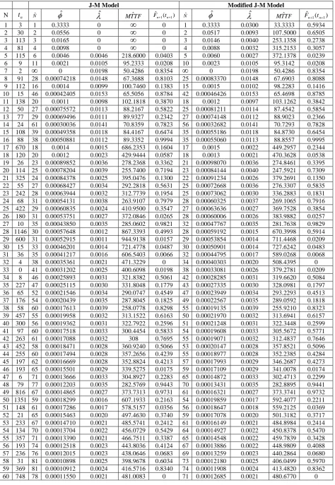
Table 1. Analysis of Musa system 1 failure data

J-M Model Modified J-M Model

N

t

n Nˆ



ˆ



ˆ

MTˆTF Fˆn1(tn1) Nˆ



ˆ



ˆ

MTˆTF Fˆn1(tn1)

1 3 1 0.3333 0



0 1 0.3333 0.0300 33.3333 0.5934

2 30 2 0.0556 0



0 2 0.0517 0.0093 107.5000 0.6505

3 113 3 0.0165 0



0 3 0.0146 0.0040 253.1358 0.2738

4 81 4 0.0098 0



0 4 0.0088 0.0032 315.2153 0.3057

5 115 6 0.0046 0.0046 218.6000 0.0403 5 0.0060 0.0027 372.1378 0.0239 6 9 11 0.0021 0.0105 95.2333 0.0208 10 0.0023 0.0105 95.3142 0.0208

7 2



0 0.0198 50.4286 0.8354



0 0.0198 50.4286 0.8354

125 10 138 0.00003727 0.00048457 2063.7 0.4049 126 0.00004061 0.00049749 2010.1 0.4130 126 1071 139 0.00003672 0.00047740 2094.7 0.1623 127 0.00003994 0.00049285 2029 0.1671 127 371 141 0.00003563 0.00049886 2004.6 0.3257 129 0.00003863 0.00051880 1927.5 0.3363 128 790 143 0.00003455 0.00051822 1929.7 0.9587 130 0.00003806 0.00051457 1943.4 0.9578 129 6150 139 0.00003672 0.00036720 2723.3 0.7046 129 0.00003822 0.00044373 2253.6 0.7709 130 3321 139 0.00003666 0.00032992 3031 0.2916 130 0.00003727 0.00043605 2293.3 0.3660 131 1045 140 0.00003608 0.00032470 3079.8 0.1897 131 0.00003664 0.00043193 2315.2 0.2441 132 648 141 0.00003555 0.00031996 3125.4 0.8271 132 0.00003607 0.00042852 2333.6 0.9047 133 5485 140 0.00003613 0.00025293 3953.6 0.2543 133 0.00003494 0.00041827 2390.8 0.3844 134 1160 141 0.00003553 0.00024870 4020.9 0.3710 134 0.00003433 0.00041408 2415 0.5378 135 1864 142 0.00003489 0.00024423 4094.4 0.6341 135 0.00003367 0.00040906 2444.6 0.8143 136 4116 142 0.00003489 0.00020934 4777 136 0.00003278 0.00040126 2492.1

Since the relationship between the reliability function )

(ti

R and the failure distribution function Fi(ti) are related byR(t_i)1F_i(t_i), the quality of reliability prediction of the models may be judged by examining the estimated failure distribution functions of the models.

From Table 1, we can see that normally the failure rate for our modified J-M model with imperfect debugging is greater than or equal to the failure rate of the J-M model. It is also noted that the MTTF is infinite for some intervals of times between failures in J-M model. So this model assumes that there are no

[image:6.595.131.464.340.536.2]

more faults in the software although faults are present in the software at that time. In our modified J-M model, the MTTF is not infinite for every interval between failures. So this is more realistic in practical sense as it implies that till then fault is remaining in the software. This is the most practical situation in software fault debugging process. When p1 and r0 i.e. for perfectly debugging procedure, our considered imperfect debugging modified J-M model approaches to the J-M model.

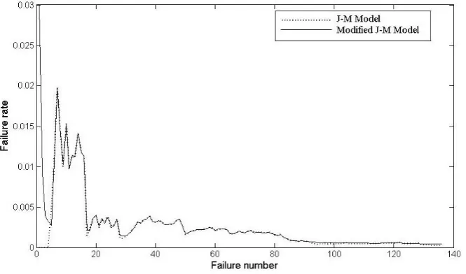
Fig 1: Failure rate as a function of failure number

A plot of failure rate against failure number for the J-M model and the modified J-M model is shown in Figure 1. From the graph of Figure 1, we get the clear idea about the failure behavior of the two models. The failure rate is maximum at the beginning of the testing process. As the fault content of the software is decreasing i.e. the failure number is increasing, the failure rate of our model is decreasing. This practical event occurs at the time of debugging.

4.1.2

Prediction analysis

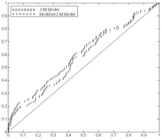
In order to compare the quality of prediction of the two models, we consider the sequences of probabilities for T_i t_i. Let uiFˆi(ti). If each of the estimated Fˆ is equal to the i true_Fi, the sequence {u_i} should look like a realization of independent uniform U(0,1) random variables [19,20,21]. We can examine the quality of each model by plotting the

sample distribution function of the i

u's and comparing it with the distribution function of U(0,1), which is the line of unity slope through the origin. We use the quantile-quantile plot [4] which is a plot of the order set of n number of u_i's against

n

[image:7.595.163.436.80.316.2]

Fig 2: Quantile-quantile plot of the data in Table 1

The quantile-quantile plot of the data in Table 1 is shown in Figure 2. The KS distance is 0.165 for the J-M model, and 0.14 for the modified model. The results show that the modified model yields a better prediction in this case.

4.2

Sensitivity Analysis of the Proposed

Model

To study the performance of our modified J-M model with imperfect debugging, sensitivity analyses have been presented graphically on the different values of p and rkeeping q as

constant. First, we consider the fixed value of q at 0.05 and the values of p and r are taken as follows:

0.94 and 0.01; 0.92 and 0.03; 0.9 and 0.05

[image:7.595.127.469.454.676.2]

p r p r p r

Fig 3: Failure rate against failure number for different values of p and r

A plot of failure rate versus failure number for the above different values of p and r of the modified J-M model is shown in Figure 3. From the graph, we can see that the failure rate is maximum for p0.9 and r0.05. But as p is

[image:8.595.155.452.82.318.2]

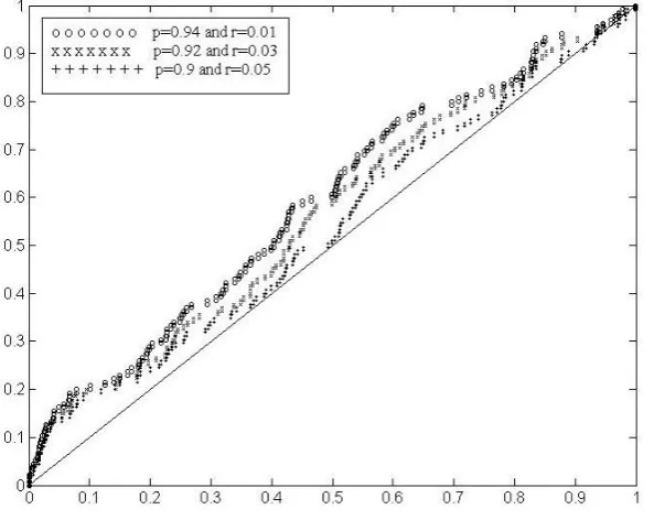
Fig 4: Quantile-quantile plots for different values of p and r

Quantile-quantile plots for the different values of p and ron the fixed value of q at 0.05 of our modified J-M model are shown in Figure 4.

Now we show the KS distances for the different values of q keeping it constant for the different values of p and r in Table 2.

Table 2. KS distances for different values of p and r for different value of q

From Table 2, we can see that for fixed value of q, as p is decreasing and r is increasing, the KS distance is decreasing. So we get better predictions as p is decreasing and r is increasing for some fixed value of q. Again, for fixed value of r, as p is increasing and q is decreasing, the KS distance is increasing. It is also noted that for fixed value of p, as q is decreasing and r is increasing, the KS distance is decreasing. So in this case we also get better predictions. From Table 2, it is clear that we get better predictions in our model for the smaller value of (p-r). In reality, the value of (p-r) is less than 1 and it decreases in most of the cases of debugging process during testing. So our model excellently predicts the software reliability in practical sense.

5.

CONCLUSION

We develop a modified J-M model which assumes the imperfect debugging process in fault removal activity during the testing phase. In our proposed model, we assume that whenever a failure occurs, the detected fault is not perfectly removed and there is a chance of raising new fault/s. We consider that the perfect debugging probability, the imperfect debugging probability and the probability of arising new fault are independent of the testing time. A set of failure data is given for illustration. From the experimental results, we have seen that the failure rate is normally high for our modified J-M model. So we need to increase the probability of perfect

debugging and to decrease the probability of raising new fault/s during the fault removing process. Again, the difference between the probability of perfect debugging and the probability of raising new fault/s should be decreased to get better software reliability prediction. The experimental results also show that our proposed model yields a better prediction than the J-M model.

6.

ACKNOWLEDGEMENTS

The authors wish to acknowledge the financial support given to this work through the research project (No. 25(0191)/10/EMR-II) by the Council of Scientific and Industrial Research, New Delhi, India.

7.

REFERENCES

[1] Lyu, M.R. 1996. Handbook of Software Reliability Engineering. McGraw-Hill.

[2] Musa, J.D., Iannino, A., and Okumoto, K. 1990. Software Reliability: Measurement, Prediction, Application. McGraw-Hill.

[3] Jelinski, Z. and Moranda, P.B. 1972. Software reliability research, Statistical Computer Performance Evaluation. Academic Press: New York, 465-484.

For q=0.07 For q=0.05 For q=0.04

p R KS distance p r KS distance p r KS distance 0.92 0.01 0.140078 0.94 0.01 0.155263 0.95 0.01 0.161781

[image:8.595.138.460.412.496.2]

[4] Littlewood, B. 1987. How good are software reliability predictions?. Software Reliability: Achievement and Assessment. Blackwell Scientific Publications. 154-166. [5] Musa J.D. 1975. A theory of software reliability and its

application. IEEE T. Software Eng. 1(3), 312-327. [6] Goel, A.L., and Okumoto, K. 1979. Time dependent

error detection rate model for software reliability and other performance measures. IEEE T. Reliab. R-28(3), 206-211.

[7] Yamada, S., Ohba, M. and Osaki, S. 1983. S-shaped reliability growth modeling for software error detection. IEEE T. Reliab. R-32(5), 475-484.

[8] Ohba, M. 1984. Software reliability analysis models. IBM J. Res. Dev. 28(4), 428-443.

[9] Goel, A.L. 1985. Software reliability models: assumptions, limitations and applicability. IEEE T. Software Eng. SE-11(12), 1411-1423.

[10]Kapur, P.K., and Garg, R.B. 1990. Optimal release policy for software reliability growth models under imperfect debugging. Oper. Res. RAIRO. 24(3), 295-305.

[11]Chang, Y.C., and Liu, C.T. 2009. A generalized JM model with applications to imperfect debugging in software reliability. Appl. Math. Model. 33, 3578-3588.

[12]Shyur, H.J. 2003. A stochastic software reliability model with imperfect-debugging and change-point. J. Syst. Software. 66(2), 135-141.

[13]Kapur, P.K., Singh, O.M.P., Shatnawi, O., and Gupta, A. 2006. A discrete NHPP model for software reliability growth with imperfect fault debugging and fault generation. Int. J. Perform. Eng. 2(4), 351-368.

[14]Prasad, R.S., Raju, O.N., and Kantam, R.R.L. 2010. SRGM with imperfect debugging by genetic algorithms. Int. J. Software Eng. Appl. 1(2), 66-79.

[15]Raju, O.N. 2011. Software reliability growth models for the safety critical software with imperfect debugging. Int. J. Comput. Sci. Eng. 3(8), 3019-3026.

[16]Xie, M. Dai, Y.S. and Poh, K.L. 2004. Computing System Reliability Models and Analysis. Kluwer Academic Publisher.

[17]Kremer, W. 1983. Birth-death and bug counting. IEEE T. Reliab. R-32(1), 37-47.

[18]Musa, J.D. 1980. Software Reliability Data. Data & Analysis Center for Software.

[19]Dawid, A.P. 1984. Statistical theory: the prequential approach. J. Roy. Stat. Soc. A. 147, 278-292.

[20]Pham, H. 2006. System Software Reliability. Springer. [21]Bittanti, S. 1988. Software Reliability Modelling and