Estimation of the parameters of a linear expenditure system (LES) demand function for a small African economy

Munich Personal RePEc Archive

Estimation of the parameters of a linear

expenditure system (LES) demand

function for a small African economy

Nganou, Jean-Pascal

World Bank

8 August 2005

Online at

https://mpra.ub.uni-muenchen.de/31450/

Estimation of the Parameters of a Linear Expenditure System (LES) Demand

Function for a Small African Economy

Jean-Pascal N. Nganou1 World Bank

Abstract:

The validity of the key behavioral parameters used in the calibration process of computable general equilibrium (CGE) models remains a debated issue in the CGE literature. CGE modelers prefer to borrow from the handful of estimates available in the literature rather than estimating these parameters empirically. The dearth of data is often mentioned as the major reason for compromises to the empirical basis for the parameters used in CGE models. While the empirical literature on demand elasticities based on household expenditure surveys has been relatively available for both developed and developing countries, it remains lacking for African countries. This paper uses a seemingly unrelated regressions method to estimate own-price and income elasticities, as well as Frisch parameters for households whose consumption behavior is described by a Linear Expenditure System (LES) demand function. All the parameters estimated are intended for use in a Lesotho CGE model. The estimation results are generally consistent with the theory predictions.

Keywords: CGE; Demand System (LES); Seemingly Unrelated Regressions (SUR); Africa; Lesotho

1

1 Introduction

The validity of the key behavioral parameters used in the calibration process of computable

general equilibrium (CGE) models remains a debated issue in the CGE literature. CGE

modelers prefer to borrow from the handful of estimates available in the literature rather than

estimating these parameters empirically. The dearth of data is often mentioned as the major

reason for compromises to the empirical basis for the parameters used in CGE models. The

empirical literature on demand elasticities based on household expenditure surveys has been

relatively available for both developed and developing countries (e.g., Lluch, Powell, and

Williams (1977), Tulpule and Powell (1978), Creedy (1996)). However, no such study exists

for Lesotho.

The purpose of this paper is to address some of the criticisms leveled against the use of

parameters taken from the literature in CGE models. We estimate parameters of a linear

expenditure system (LES) demand function, including elasticities of expenditures, own-price

elasticities, and Frisch parameters, all intended for use in the Lesotho CGE model (Nganou,

2005).

2. The Data

For the estimation of LES parameters, the 1994/95 Lesotho Household Expenditures Survey

(HES) of the Lesotho Bureau of Statistics was used to derive expenditure levels. The

commodities for which data were available in the HES were re-categorized to match the

commodities classification provided in the Lesotho SAM (STLESAM). Thus, Lesotho

households direct most of their spending to the following nine commodities: Agriculture,

Food, Beverages and Tobacco, Textiles, Utilities, Private Services, Government Services,

Table 1 presents the descriptive statistics for commodities expenditures and consumer price

indices for each category of household. The data set contains a maximum of 1932

observations for urban households and 2628 observations for rural households. In general,

expenditure and price levels are higher for urban households than their rural counterparts. As

expected, the average annual expenditure amounts to 91,721.86 Maloti for urban households

compared to only 35,185.76 Maloti for rural households. Financial services (including all

forms of informal sources of finance such as through funeral homes) seem to be the most

purchased service for urban households (12,000 Maloti on average) whereas rural households

consumed mostly textile products (10,160 Maloti). It was not useful to break the data set

down into several sub-samples according to income and location to agree exactly with the

disaggregation provided in the STLESAM because the number of observations was

significantly smaller for some sub-samples. Prices data are also needed to estimate LES

parameters. This study uses the 2000 Consumer Price Index (CPI) series by commodities and

location (rural and urban) provided by the Lesotho Bureau of Statistics as price variables

(1997 was the base year)2 .

TABLE 1 HERE

3. Estimation of Parameters

Zellner’s SUR method was used to estimate LES parameters because efficiency gain can be

achieved by combining each demand equation as a system.

3.1 Estimating the Parameters and Elasticities of the LES Demand

3.1.1 Theoretical Background and Methodology3

In many CGE models, household preferences are derived from the maximization of Cobb

Douglas or CES utility specifications. A fundamental limitation of such functional forms for

2

The 2000 CPI were used instead of the 1994/95 CPI because the Lesotho SAM that serves as the dataset for the CGE is of 2000.

3

consumption is that they imply unitary income elasticity of demand since average and

marginal propensities to spend are constant and equal for these specifications. Another

limitation of CES specifications in consumer preferences can be seen in the case where there

are many small consumer goods. In this case, there is an excessive symmetry between goods

since the compensated own-price elasticity for each good converges on the common elasticity

of substitution between all goods (Shoven and Whalley, 1984). Unlike CES functions, linear

expenditure system (LES) utility functions assume that average propensities to spend vary

systematically with income level due to the minimum subsistence requirement imposed on

each good (Davies, 2003). To avoid such drawbacks, an interesting feature of the Lesotho

CGE model is its assumption that, each household maximizes a linear expenditure system

(LES) or Stone-Geary utility function subject to its consumption expenditure constraint.

Household h’s consumption problem under this set-up is the following:

Max





10

1

.ln

h ch ch ch

c

U  QH 







subject to the budget constraint and the Engel aggregation condition4 on the βs:

10

1

.

h c ch

c

EH PQ QH







10 1 1 ch c   



where γchand βch are the LES parameters. More precisely, the former is the marginal share of

consumption spending for household h on marketed commodity c, and the latter is the

subsistence requirement on each marketed commodity c for household h; QHch is the

4

The Engel aggregation condition requires that

household h’s consumption quantity of marketed commodity c; PQc is the price of commodity

c.

The Lagrangian for this optimization problem is as follows:

Max

10

1

.

h h c ch

c

L U  EH PQ QH



 

  _  _





Differentiating the above Lagrangian equation with respect to QHc, and after some

rearrangements of the first order conditions, yields the demand function of the household h on

commodity c which later will be estimated econometrically:

10

' ' ' 1

.

ch

ch ch h c c h

c c

QH EH PQ

PQ         _  _





It is clear from equation (1) that a household’s spending on individual commodities is a linear

function of the total consumption spending (or income) EHh. The usual interpretation of the

above demand function is that consumption has two components. The first component has

been referred to as the subsistence minima (or consumption floor), γch. The expression in

parentheses represents the residual income (supernumerary income), or, as some researchers

call it, luxury expenditures/usages. It is the remainder of income after subtracting

expenditures on the subsistence minima. The second term of the demand function is therefore

a share of supernumerary income. In fact, γch represents subsistence quantities while βch

reflects the relative contribution of each commodity to utility after subsistence has been

achieved.

For estimation purposes, it is common practice to multiply both sides of eq. (5) by PQc to

obtain a linear expenditure system of equations, so designated because expenditure is a linear

function of income and prices. The expenditure system is clearly not linear in the parameters

(γch and βch) (see Judge, Hill, Griffiths, Lutkepohl, and Lee (1988)). The corresponding

10

' ' ' 1

. . .

c ch c ch ch h c c h ch c

PQ QH PQ   EH PQ  



 

  _  _





where εch is the error term, γchand βch are the parameters to be estimated, c=c’ represents the

commodities for which sample data on prices, quantities, and income are available for the

estimation of parameters (i.e., c= Agriculture, Food, Beverages and Tobacco, Textiles,

Utilities, Private Services, Government Services, Transport, Other Manufacturing, and

Financial Services). Meanwhile, only two household categories had appropriate data (i.e., h=

urban, rural). The system represented by equation (6) can be viewed as a set of nonlinear

seemingly unrelated regression equations since it can be shown that the covariance matrix of

the system is not diagonal.

Due to the fact that the sum of expenditures should equal the total income (i.e., the sum of the

dependent variables is equal to one of the explanatory variables for all observations), the sum

of error terms for each equation of the system is equal to 0, leading to the singularity of the

covariance matrix. In such conditions, estimation procedure breaks down. To overcome this

singularity problem, it is common practice that one equation be omitted for the estimation of

the demand system (Judge, Hill, Griffiths, Lutkepohl, and Lee, 1988).

The adding-up constraint

10

1

.

h c ch

c

EH PQ QH







by difference. The choice of the omitted equation is arbitrary. Given that the estimation

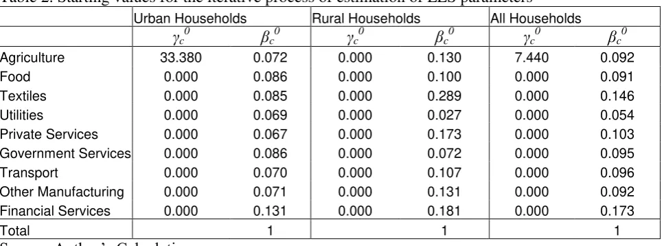
method used here is iterative, the choice of starting values is also crucial. There is no clear

rule on these values5. But as stated in Judge, Hill, Griffiths, Lutkepohl, and Lee (1988), “the

nature of the model provides some guide as to what might be good starting values for an

iterative algorithm.” For each commodity they suggest the minimum value of the quantity

demanded as a reasonable starting value for the associated γch. Also, they proposed the

5

average budget shares to be good starting values for the βch. Consequently for our purposes,

the starting values used are summarized in table 2 below.

TABLE 2 HERE

The ITSUR method available in SAS (version 9.0) was employed in the estimation of eq. (6)

with restrictions of non-negativity of coefficients imposed (i.e., γch >=0, and 0 <βch< 1).

According to Zellner (1962), seemingly unrelated regression equations (SURE) are systems

whose equations, at first examination unrelated, are in reality related through the correlation in

the errors. In short, a set of equations that has contemporaneous correlation between the

disturbances in different equations is a seemingly unrelated regression system. ITSUR

procedure adjusts for cross-equation contemporaneous correlation and consequently takes into

account the optimization process underlying the demand system. The iterative process of the

ITSUR ensures that the obtained estimates approach asymptotically those of the maximum

likelihood method. Moreover, ITSUR unlike Seemingly Unrelated Regression (SUR) is

insensitive to the excluded equation (in our case the financial services equation) (Judge, Hill,

Griffiths, Lutkepohl, and Lee, 1980)6. Breusch-Pagan and White tests for heteroskedasticity

were performed for separate equations of the system in this study. Both tests significantly

rejected the null hypothesis, indicating the presence of cross equation contemporaneous

correlation7. Thus, the set of demand equations to be estimated is a seemingly unrelated

system. Therefore, Zellner’s estimation approach (SUR) is appropriate for this purpose.

3.1.2 Estimation Results

The results of estimation are presented in Table 3 below. Interestingly, findings suggest that

the subsistence requirement parameter (γch) is higher for urban households compared to that

for their rural counterparts in the following commodities: Agriculture, Food, Utilities,

6

ITSUR iterates from initial guesstimates specified.

7

Government services, and Other Manufacturing. In most of these commodities, the value of

those parameters is double the value for rural households. The subsistence parameter for

Transport is relatively larger among rural households (M2739.90 compared to M128.68 for

urban households). This makes sense since in rural areas, given the scarcity of transport and

communication infrastructure, the subsistence levels should be higher. The subsistence

parameter for Financial Services is estimated to be zero among urban households while it is

around M2900 for their rural counterparts. In fact, in rural areas, given that funeral homes are,

in general, the only financial intermediaries (informal), households do not have many options

as compared to urban households. Findings also reveal that for urban households, the share of

supernumerary income (βch) is important toward Financial Services (38 percent), Transport

(23 percent) and Private Services (12 percent). Meanwhile, rural households spend 26 percent

of their supernumerary income on Other Manufacturing commodities, 22 percent on Private

Services (personal care, etc.), and 20 percent on Financial Services. These results suggest that

for each household group, the commodities mentioned above are luxuries. This is also

confirmed by their associated income elasticities greater than unity (see Table 5 below).

Interestingly, urban households spend more of their supernumerary income on Transport than

do rural households (4 percent). This suggests that transport and communication is a luxury in

urban areas whereas it is a necessity in rural zones.

TABLE 3 HERE

In CGE models that adopt LES demand systems to represent the consumption behavior of

households, income elasticity of each commodity and Frisch parameters for each household

category are crucial in the calibration process. The Frisch parameter is the substitution

parameter measuring the sensitivity of the marginal utility of income to income/total

expenditures. The Frisch parameter, also called money flexibility, establishes a relationship

studies) where reliable price data are difficult to be obtained and to provide good estimates of

own-price elasticities. Consequently, the relationship for directly additive preferences

proposed by Frisch (1959) and embodied in the Linear Expenditure System (LES) is often

used to derive own- and cross-price elasticities. In fact, price elasticities of demand are

determined simply by the income elasticity in conjunction with the Frisch parameter.

Moreover, relying on Frisch parameters prevent us from using own-price elasticities with

positive signs in the CGE model. Also, given the huge number of cross-price elasticities (i.e.,

n(n-1)) to be estimated, there would be an enormous saving in statistical investigation if the

Frisch parameters were used to derived those elasticities instead of making any separate

analysis for each of the cross-price elasticities (Frisch, 1959).

The formula used to derive Frisch parameters is simply the negative ratio between a

household’s total expenditures and the supernumerary income (i.e., the difference between

household income and total expenditures on subsistence requirements) at the sample means

(indicated by a bar over a variable). Frisch parameters are

10 ' ' ' 1 . h h

h _{c c h} c

EH Frisch

EH PQ 

        



Similarly, we calculate Marshallian own-price and expenditure elasticities at the sample

means. The Marshallian own-price elasticities are





    (8)

The expenditure/income elasticities are

. . h ch ch ch ch EH PQ QH 

After estimating the LES parameters, we use a feature of the SAS software (i.e., “Estimate”)

to compute/derive own-price, income/expenditure elasticities, as well as Frisch parameters for

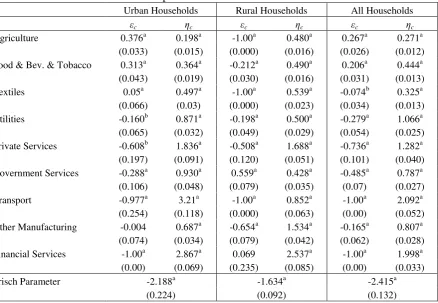
the two household subcategories and the entire sample. These results are presented in Table 4

along with associated standard errors.

With regard to own-price elasticities, we observe that the demand for the majority of

commodities listed is either price inelastic or unitary elastic in some cases. There are some

commodities whose price elasticities have the wrong sign (positive). More specifically, for

urban households, findings indicate negative own-price elasticities for all commodities, with

few exceptions (Agriculture, Food, and Textiles), as predicted by the neoclassical consumer

theory. While the demand for Financial Services is unitary elastic, the price elasticity of

demand for Transport nears unity. Other Manufacturing and Utilities sectors have the lowest

own-price elasticities (-0.004 and -0.160) for urban households. It is worth mentioning that

Textiles and Other Manufacturing are the only commodities for urban households whose price

elasticities are not statistically significant. Among rural households, the demand for

Agriculture, Textiles, and Transport is statistically significant unitary elastic, which means

that a unit increase in the price of those commodities leads to a unit reduction in their

respective quantities demanded. Meanwhile, rural households’ demand for Government

Services and Financial Services has own-price elasticities with a positive sign, which

contradicts neoclassical consumer theory predictions. However, while the latter is not

statistically significant, the former certainly is, which seems to suggest that Government

Services is a Giffen “good” for rural households. It could also be the case that the estimated

consumption behavior of Basotho households8. Given that the own-price elasticity for

Financial Services and Textiles is not statistically significant among rural and urban

households respectively, it suggests that the demand for those commodities is vertical for both

household groups. This finding indicates that a marginal increase in the price of those

commodities leaves its demand unchanged. For the entire sample (across all households), the

demands for Agriculture and Food commodities have statistically significant positive

own-price elasticities (wrong sign).

TABLE 4 HERE

On the other hand, findings suggest that all the commodities listed are normal goods, given

that their income elasticity is positive in sign. For urban households, Agriculture has the

lowest income elasticity, followed by Food, Textiles, and Other Manufacturing (0.198-0.687).

Also, given that the income elasticity for all other commodities, except Private Services,

Transport, and Financial Services, is positive but less than one, those commodities are

necessities for urban households. Meanwhile, among rural households, the income elasticity

for Private Services, Other Manufacturing and Financial Services is greater than one,

suggesting that those commodities are luxuries. Other Manufacturing is a luxury for rural

households whereas it is a necessity for urban households. This makes sense since household

appliances, which constitute part of Other Manufacturing, can be thought of as luxury goods

in rural areas. In fact, rural households in general do not use modern household appliances;

rather, they resort to rudimentary methods/tools. The same contrast can be drawn for

Transport and Communication, which is a luxury for urban households and a necessity for

rural households. Interestingly, the income elasticities on Agriculture, Food, and Textiles are

larger for rural households. For instance, an increase of 100 units in the income of urban

households leads to an increase of 20 units in their demand for Agriculture. A similar increase

8

in the income of rural households causes an increase of 48 units in their demand for

Agriculture. In sum, Agriculture, Food, and Textiles are more necessities for rural households

than they are for their urban counterparts.

4 Conclusion

The objective of this paper was to estimate some key parameters intended for use in the CGE

model for Lesotho. Using Household Expenditures Survey (HES) data, ITSUR methods were

utilized in the estimation of own-price and income elasticities, and the derivation of Frisch

parameters. The estimated coefficients were generally robust. We found that although

Agriculture, Food, and Textiles can be thought of as necessity goods for both rural and urban

households, a marginal change in the demand of these products will have a greater effect on

rural households.

(American University). The author is also indebted to Sherman Robinson (University of Sussex) for his comments on a previous version of this paper. An earlier version of the paper

was presented at the International Conference “Input-Output and General Equilibrium: Data,

Modeling, and Policy Analysis”, Brussels (Belgium), September 2-4, 2004. Electronic comments addressed to [email protected]. The usual disclaimer applies.

REFERENCES

Creedy, John (1996) Measuring the Welfare Effects of Price Changes: A Convenient Parameter Approach, Research Papers of The University of Melbourne (536), 1–31.

Frisch, Ragnar (1959) A Complete Scheme for Computing All Direct and Cross Demand Elasticities In A Model with Many Sectors, Econometrica27, pp.

Judge, George G., R. Carter Hill, William E. Griffiths, Helmut Lutkepohl, and Tsoung-Chao Lee (1980) The Theory and Practice of Econometrics (New York, USA).

Judge, George G., R. Carter Hill, William E. Griffiths, Helmut Lutkepohl, and Tsoung-Chao Lee (1988) Introduction to the Theory and Practice of Econometrics (New York, USA).

Lluch, C., A. A. Powell, and R. A. Williams (1977), Patterns in Household Demand and Saving (Oxford: Oxford University Press for the World Bank).

Nganou, Jean-Pascal Nguessa (2005) A Multisectoral Analysis of Growth Prospects for Lesotho: SAM-Multiplier Decomposition and Computable General Equilibrium Perspectives Unpublished Ph.D. Thesis, American University, Washington, DC (US).

Tulpule, A. and A. A. Powell (1978) Estimates of Household Demand Elasticities for the ORANI Model, IMPACT Project Working Paper (OP-22).

Table 1. Descriptive Statistics (means) for Commodities Expenditures and Consumer Price Indices by Household type

Urban Households Rural Households All Households

Obs. Expenditures CPI Obs. Expenditures CPI Expenditures CPI

Agriculture 1900 6563.45 1.47 2326 4573.57 1.43 5468.22 1.45

Food & Bev. & Tobacco 1932 7886.18 1.53 2525 3504.49 1.48 5403.84 1.50

Textiles 1932 7780.45 1.33 1077 10159.18 0.57 8631.86 0.89

Utilities 1932 6287.66 1.29 2628 950.726 1.35 3211.9 1.32

Private Services 1932 6155.31 1.30 1503 6073.81 0.74 6119.65 0.98

Government Services 1932 7856.48 1.20 1374 2529.74 0.63 5642.64 0.87

Transport 1932 6457.14 1.50 799 3768.5 0.44 5670.53 0.89

Other Manufacturing 1932 6476.14 1.37 2449 4602.59 1.30 5428.82 1.33

Financial Services 1932 12007.06 1.30 866 6355.26 0.43 10257.79 0.79

Total Expenditures 1932 91721.86 2628 35185.76 59139.21

Source: Author’s calculations

Table 2. Starting values for the iterative process of estimation of LES parameters

Urban Households Rural Households All Households

γc 0 _β c 0 _γ c 0 _β c 0 _γ c 0 _β c 0

Agriculture 33.380 0.072 0.000 0.130 7.440 0.092 Food 0.000 0.086 0.000 0.100 0.000 0.091 Textiles 0.000 0.085 0.000 0.289 0.000 0.146 Utilities 0.000 0.069 0.000 0.027 0.000 0.054 Private Services 0.000 0.067 0.000 0.173 0.000 0.103 Government Services 0.000 0.086 0.000 0.072 0.000 0.095 Transport 0.000 0.070 0.000 0.107 0.000 0.096 Other Manufacturing 0.000 0.071 0.000 0.131 0.000 0.092 Financial Services 0.000 0.131 0.000 0.181 0.000 0.173

Total 1 1 1

Source: Author’s Calculations

Table 3. Estimation Results of parameters of the LES Demand System

Urban Households Rural Households All Households

γc βc γc βc γc βc

Agriculture 6115.67a 0.014a 3696.41a 0.089a 4745.30a 0.025a Food & Bev. & Tobacco 6993.31a 0.031a 2864.39a 0.072a 4446.53a 0.041a Textiles 6415.99a 0.042a 7919.98a 0.09a 6307.41a 0.048a Utilities 4345.50a 0.06a 782.58a 0.02a 1903.72a 0.058a Private Services 2126.28b 0.123a 2192.90a 0.216a 1436.41a 0.133a Government Services 5046.26a 0.080a 2103.88a 0.020a 2610.10a 0.075a Transport 128.68 0.230a 2739.90a 0.040a 0.00 0.201a Other Manufacturing 4966.32a 0.050a 2020.60a 0.261a 3586.74a 0.074a Financial Services 0 0.38 2916.91a 0.20 0.00 0.35 Source: Author’s Calculations.

Note. a = significant at 1 percent level, b= significant at 5 percent level; γc is the subsistence requirement

Table 4. Own-Price and Income/Expenditures Elasticities of the LES Demand

Urban Households Rural Households All Households

εc ηc εc ηc εc ηc

Agriculture 0.376a 0.198a -1.00a 0.480a 0.267a 0.271a

(0.033) (0.015) (0.000) (0.016) (0.026) (0.012)

Food & Bev. & Tobacco 0.313a 0.364a -0.212a 0.490a 0.206a 0.444a

(0.043) (0.019) (0.030) (0.016) (0.031) (0.013)

Textiles 0.05a 0.497a -1.00a 0.539a -0.074b 0.325a

(0.066) (0.03) (0.000) (0.023) (0.034) (0.013)

Utilities -0.160b 0.871a -0.198a 0.500a -0.279a 1.066a

(0.065) (0.032) (0.049) (0.029) (0.054) (0.025)

Private Services -0.608b 1.836a -0.508a 1.688a -0.736a 1.282a

(0.197) (0.091) (0.120) (0.051) (0.101) (0.040)

Government Services -0.288a 0.930a 0.559a 0.428a -0.485a 0.787a

(0.106) (0.048) (0.079) (0.035) (0.07) (0.027)

Transport -0.977a 3.21a -1.00a 0.852a -1.00a 2.092a

(0.254) (0.118) (0.000) (0.063) (0.00) (0.052)

Other Manufacturing -0.004 0.687a -0.654a 1.534a -0.165a 0.807a

(0.074) (0.034) (0.079) (0.042) (0.062) (0.028)

Financial Services -1.00a 2.867a 0.069 2.537a -1.00a 1.998a

(0.00) (0.069) (0.235) (0.085) (0.00) (0.033)

Frisch Parameter -2.188a -1.634a -2.415a

(0.224) (0.092) (0.132)

Source: Author’s Calculations.