A Theoretical Foundation for Count Data Models

Munich Personal RePEc Archive

A Theoretical Foundation for Count

Data Models

Hellerstein, Daniel and Mendelsohn, Robert

Economic Research Service, USDA

1993

Online at

https://mpra.ub.uni-muenchen.de/25265/

A

Theoretical

Foundation

for

Count

Data

Models

Daniel Hellerstein and Robert Mendelsohn

The paper develops a theoretical foundation for using count data models in travel cost analysis. Two micro models are developed: a restricted choice model and a repeated discrete choice model. We show that both models lead to identical welfare measures.

Key words: count data, repeat discrete choice, travel cost analysis, welfare analysis.

For several decades, economists have used the annual demand for trips in order to measure the nonmarket value of recreation sites. Two fea- tures of trip demand functions complicate their estimation: trip demand is nonnegative and oc- curs in integer quantities. The fact that trip de- mand cannot be negative results in a censored (at zero) data set; failure to account for censor- ing leads to biased estimation. The integer na- ture of trip demand, when continuous models are estimated, can also lead to biased results.

A variety of techniques have been developed to deal with these problems, including models incorporating truncated error distributions, ran- dom utility models, discrete/continuous models, and repeated discrete choice models.' In this pa- per we explore the use of count data estimators, such as the Poisson model, to embody the rec- reational demand for trips. Poisson models are becoming increasingly common (Hellerstein, Creel, and Loomis; Smith, Shaw, Terza, and Wilson). In addition, a variety of count model extensions to the Poisson have been recently de- veloped, providing analysts with a menu of ro-

bust and flexible estimators (see Hausman, Hall, and Griliches, or Cameron and Trivedi).

Although the attractive econometric proper- ties of count estimators are well understood, a theoretical foundation for their use in welfare analysis has not yet been presented. In partic- ular, the link between an individual consumer's optimization problem and a count estimator has not been drawn. Without a theoretical founda- tion, it is not clear how to interpret count models. More importantly, it remains ambiguous how to apply the results of count estimators of demand to welfare analysis. For example, it is unclear how to value recreation sites on the basis of a count demand model for trips.

Our paper addresses this shortcoming by de- veloping two theoretical frameworks for count demand models. The first model modifies a standard, continuous demand model to account for a constrained integer choice set. The second approach is based on a discrete choice model which is then repeated over time. Welfare mea- sures based on both these underlying models are derived, and are shown to yield the same for- mula for measuring consumer surplus.

The Restricted Choice Model

We begin with the standard assumption that each individual maximizes utility subject to an in- come constraint. We add an additional con- straint, however, that the choice of trips, X1, must be a nonnegative integer. In addition, we as- sume that at the beginning of the season each individual chooses X, (the number of trips) as well as the quantity of a vector of other goods (X2) _{ing Pudney (p. 94), utility maximiza-}

Following Pudney (p. 94), utility maximiza- Daniel Hellerstein is a natural resource economist with the Eco-

nomic Research Service, Resources and Technology Division; Rob- ert Mendelsohn is a professor at the Yale School of Forestry and Environmental Studies.

The views in this paper are those of the authors and do not nec- essarily reflect the views of the U.S. Department of Agriculture or Yale University.

Review coordinated by Richard Adams.

'Continuous demand models have been estimated with truncated error distributions (Shaw). Random utility models have been esti- mated as though the choice was purely discrete (Smith and Kaoru, Hanneman [1984a]). Continuous models have been appended to discrete models (Heckman, Bockstael et al.); with the discrete choice stage used to predict the probability of "participation," and the con- tinuous stage used to estimate the amount of goods selected, given participation. Repeated discrete models have been explored with fixed number of choice opportunities (Morey, Shaw, and Rowe), and discrete choice has been applied given the prior number of trips taken (Adamowicz, Jennings, and Coyne).

Hellerstein and Mendelsohn Count Data Models 605 tion can be expressed as a function of X, and

X2, where X2 is a vector of all other goods as-

sumed to be available in any quantity. For- mally, each individual solves

(1)

max [U(X, X2, ; 3)P * X = pixi + P2X2

_Y]

XIEl, X2

where P (the vector of prices) is divided into P1 (the price of the indivisible good) and P2 (a vec- tor of prices of other goods), E are unobservable factors specific to an individual, and Y is in- come.2 Since X, is restricted to I (I = 0, .. .), this can be rewritten as

(2)

max{max U[(XI, X2, E; _3)1P2X2 = _{Y- PIX1]}}

XIEI X2

Taking the dual of (2), the expenditure function can be written as

(3)

E[P,, P2, _{; Uo] = minX{PX* +} [min(P2X2)]

X1 X2

s.t. U(X *, X2, ; _{/3) = U0, X*= X1}}

where Uo is a reference level of utility.

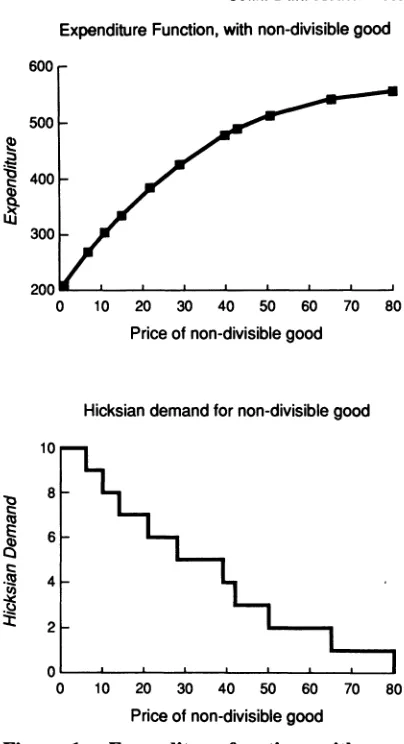
Equation (3) highlights the two components of the decision making process: how much of X, to consume and how much of X2 to buy. Since

X, can only be changed in infra-marginal amounts, the compensated demand for X1, H(P,,

P2, E, _U0) = _aE/aPI, will be constant over dis-

crete ranges of the expenditure function, with discrete jumps at prices that define the end- points of these ranges. As illustrated in figure 1, the expenditure function will be piecewise linear, and the compensated demand will be a step function.

If repeated observations on a single individual could be obtained, each observation differing only in price, it would be possible to determine the step-function comprising the compensated de- mand curve for an indivisible good. In actual circumstances, such a highly controlled sample is rarely available. Instead, price variation oc- curs across individuals, where each individual in the sample possesses a unique set of unob- servable (E) factors. At any price, these factors (ceteris paribus) determine the quantity each in- dividual consumes.

Estimating demand relationships with such data, the analyst can at best determine proba-

Expenditure Function, with non-divisible good

600

500

400

300

200

0 10 20 30 40 50 60 70 80

Price of non-divisible _good

Hicksian demand for non-divisible _good

10

8

0

2 -

0 10 20 30 40 50 60 70 80

Price of non-divisible _good

Figure 1. Expenditure function, with non- divisible good. Hicksian demand for non-div- isible good

bilities of observing a level of demand, given prices, income, and other observable variables. One means of summarizing these probabilities is through a probability density function. Viewed in this manner, estimation of a demand curve is an exercise in computing the parameters of a probability density function. These parameters will vary as prices vary; hence, the probability of observing a particular level of demand will change as prices vary.

It is interesting to consider the estimation of continuous demand curves. The random com- ponent (E) is often included as a demand shifter; for example, in the linear model of demand for a good Q, Q = _{Xp + E. Alternatively, one can} assume that, conditional on observed prices, de- mand will be distributed according to some con- tinuous probability distribution. For example, demand can be postulated to follow a normal

2

606 August 1993 Amer. J. Agr. Econ.

distribution: Q - N(XP,

0-2); with the XP of the linear model now interpreted as the location pa- rameter of a normal distribution, and 0-2 de-

scribing the variance of e across the population. This interpretation of continuous demand is es- sentially the same as the interpretation of the de- mand for indivisible goods offered above.

For indivisible goods, a probability distribu- tion defined only over the nonnegative integers is required. One such candidate for this distri- bution is the Poisson. The Poisson probability distribution is a single parameter distribution (A), with probability density function (PDF) defined as

e-A"A

(4) prob(Q = n)= ; n = 0, 1, .. ., n!

where Q is a potential integer outcome. The A parameter of the Poisson is equal to the mean, E[Q], and the variance, o-2[Q], of Q. Typically, the A parameter is modeled as a function of prices and income, such as A(P, Y; P). For applied work, an exponential form for A is usually em- ployed: for example, A = exp(/30 + OPP + WY), where 0 is a vector of coefficients to be esti- mated.

Estimation of a Poisson model,3 using data on demand for an indivisible good (such as trips to a recreational site), yields coefficient estimates which can be used to compute values of A(P, Y; 0). As a continuous quantity, A(P, Y; P) does not represent an obtainable level of demand. Rather, A(P, Y; 0) parameterizes the distribution of demand (over the nonnegative integers) for individuals facing prices P and income Y.

Welfare analysis is often conducted by com- puting a consumer surplus (as an approximation to a compensating variation) by integrating un- der a demand curve. With count models, the es- timated function is a probability distribution of trips. Taking the expectation of this distribution yields an expected response (number of trips) at every price. By integrating underneath this ex- pected response, a measure of the expected value of consumer surplus is obtained.

Formally, the expected value of the consumer surplus (E[CS]), given a price change in good

1 from Pi, to P~b, is

(5) lb

E[CS] = _{[f(s) T(p, P2, Y,} E; _{3)] de dp} JPa E

where T( ) is an individual's demand curve for the indivisible good (e.g.; trips), which will be a step function with exact shape dependent on

E. _{The E argument in T, which has a range of}

support of E and a PDF equal to f(e), is meant to capture the influence that unobservable fac- tors have on trip taking decisions.4 Rearranging (5) yields

Plb

(6)

_{AI, (p,}

Y; P)dp = E[CS]

in which we use the assumption that trip de- mand is, ceteris paribus, Poisson distributed, and the mean of the Poisson equals A(P,, P2, Y; 1). Note that if one estimates A = eXt (X = P, Y) and Plb equals infinity, equation (6) yields the standard result of E[CS]= -A/Pp.

Summarizing this section, we show that when using count models to estimate trip demand, computation of the expectation of consumer sur- plus is obtained by integrating under the ex- pected value of demand. If one assumes that de- mand, at any given price, follows a Poisson distribution, then the expected value of demand will equal A. This result holds even though the expected value of demand may not be an integer and thus cannot be obtained by a single indi- vidual.

It is interesting to contrast this to continuous models, where consumer surplus measurement techniques dictate use of observed demand (Bockstael et al.) to estimate consumer surplus for individuals in a sample. A common pre- sumption is that random and unobservable fac- tors (e) effect demand in an additive (or multi- plicative) fashion. The count model, in contrast, estimates the distribution of trips from which any individual draws; with random factors incorpo- rated in a parametric fashion rather than as a residual.

The Repeated Discrete Choice Model

As an alternative to the restricted choice frame- work presented above, count models can also be derived from repeated discrete choices. At each choice interval, the consumer can make a bi- nomial (zero/one) choice to consume or not. For example, each day, the recreator can choose whether to take a trip to a site or to engage in some other activity. The count model can then 3 Estimation of a Poisson, and other count models, is usually

accomplished with maximum likelihood techniques. A growing number of econometric packages directly support count model es- tilnation; such as LIMDEP, SHAZAM, and GRBL.

Hellerstein and Mendelsohn Count Data Models 607 be derived from a repeated application of these

discrete choices.

A simple conditional utility model is adopted to reflect the discrete choice of consuming or not:

(7) V* = max(Vj(Pj, Y, Ej); J = {0, 1} JEJ

where V* is realized utility and Vj(Pj, Y, Ey) is the utility associated with the choice of good j, given the price of obtaining activity j (Py), the individual's income (Y), and a random shock term unique to good j (Ey). Good one (j = 1, e.g. the site is visited) is selected when the choice of good one yields greater utility than realized when good zero (j = 0, e.g. not visiting the site) is chosen.

When the random shocks, E = {Eo,

El}, change over time, equation 1 becomes

V* = max(Vj(Pj, Y, Ej,) J = {0, 1}.

Hence the consumer's choice will depend on the realization of E, = {Eo,, _El,}.5 Furthermore, if we assume (without loss of generality) that Po equals zero, on a given day t there is a probability irt(P,, Y) that the good one will be chosen (the site will be visited), and a probability 1 - ir,(P1, Y) that it will not.6 If chosen, a quantity of one is de- manded, otherwise the quantity demanded is zero. If P, is constant across time, and the distri- bution of E is independent and identically dis- tributed (iid) across time, ir, will be constant over

time. Therefore, the outcome of the repeat dis- crete choices faced by the consumer can be modeled as a series of iid draws. Total number of draws over the course of the season will have a binomial distribution. As the number of draws increases, and the probability of choice de- creases proportionally, this binomial distribu- tion will asymptotically converge to a Poisson distribution (Mood, Graybill, and Boes). In other words, the count of the number of days (within a year) that good one is chosen will be asymp- totically distributed as a Poisson random vari- able.

It is important to note that the Poisson distri- bution of outcomes is not dependent on the ex-

act distribution of

ir. However, the functional form of the Poisson parameter, A(P, Y; P), does depend on ir. For example, it can be shown that if each discrete choice yields a logit distribution for _ir, and the choice probability is small and constant across time, the functional form for A will asymptotically equal exp(f30 + _IpP + p y).7

To analyze welfare calculations in the repeat discrete choice context, the results of Hanemann 1984 (b) are adapted. We first focus on a single choice opportunity (say, a single day), and de- fine a measure of the value of the good (say, a recreational site). For a given day t, site value is based on a compensating variation (CV,), de- fined as

(8a) CV, = min s.t. V,(PO, P, + CV, Y, El,) cv

-- Vo(Po, P,, Y, E0rt) Because E is stochastic, CVt is also stochastic. Thus, it is of interest to examine the expected value of CV,,

(8b) _{E[CV,] = .}

CVft(CV)dCV

-=

_{(1 - Ft(CV))dCV}

where f,(CV) and F,(CV) are the probability density function and cumulative distribution function of CV, (respectively).8

When Vo(Po, P1, Y, Eot) ?

VI(P0, P1, Y, _Elt),

good one is not chosen and CV, equals zero. Therefore

F(0O) = prob(Good 1 not chosen on day t) = 1 - prob(Good 1 chosen on day t) = 1 - ir,(P1, Y), (by assumption). Similarly, for any nonnegative quantity A, Ft(A) will equal the probability of good one not being chosen when its price equals P, + A, which equals 1 - 'i,(P1 + A, Y). Substituting these results for F(0O) and F,(A) into (8b) yields

(8c)

E[CVt]

=

f

,t(pl

+ A, Y)dA

=

f

_r(p,

5 For example, if Vj( ) ; V0( ) and P1 = Po, and if on day t = T, e1, is very large and E, is very small, then good one will be chosen. Alternatively, if on day t = y, e~, is very small and coy is very large, then good zero will be chosen.

6 _{For example, if utility is of the form V + e, good one (j = 1)}

is chosen when co < el + V, - Vo. Given that V, and Vo are non- stochastic, different choices occur as el and co vary. The classic case of logit probabilities occurs when the elements of e1 and Co are

independently drawn from a type I extreme value distribution (Maddala, ch. 3).

7 The logit assumes that Vi = XfI + ei, where X is a vector of prices, etc., and ei follows a type I extreme value distribution. See the appendix for a further discussion of these results.

8 _{See Hanemann (1984b), equation 26, or Mood, Graybill, and}

608 August 1993 Amer. J. Agr. Econ.

Lastly, it is readily shown that the E[CV,] equiv- alent to the change in the price of good one from Pa to Pb equals

(9) E[CV,] = J

_'n

Given that _ir, is constant over time, the ex- pected value of the total compensating variation (CV) over an entire period (say, over a year consisting of T days) will be

(10) _{E[CV] = E ZICV} =E[CVj]

=

Y)dp =

Z

_t(p,

t P

P

Because the Poisson process defines A as the re- sult of many small probability events, it im- mediately follows that9

(11) pb Tb

E[CV] = _E (p, Y)dp A(p, Y)dp.

Therefore, the price integral over the Poisson parameter, A(P, Y), is a legitimate approxima- tion to the compensating variation. Further- more, as with the restricted choice model, if A = exp(XP) is used and Pb = 00, E[CV] will equal

Extensions

The assumption that the resulting distribution of trips is Poisson need not always hold. In partic- ular, the assumption of equality between the ex- pected value, E[Q], and the variance of the dis- tribution, &o2[Q], is stringent. The Poisson relationship, A = A(P, Y; P), also does not con- tain an error component."

To relax these assumptions, a variety of ex- tensions to the Poisson are available. An espe- cially appealing alternative is the Negative Bi- nomial count model. Formally (following Cameron and Trivedi), if Q is a Poisson random variable with parameter A, and A is distributed as a gamma random variable y(A; g, V), then Q is distributed as Negative Binomial random variable with E[Q] = u and var[Q] = g + gt2/v.

The relaxation of statistical restrictions of- fered by the Negative Binomial can be further extended. Specifically, the Poisson (and Nega- tive Binomial) are examples of the class of lin- ear exponential functions, and it can be shown that as long as the specification of the mean is correct, linear exponential functions will be ro- bust to misspecification (Gourieroux, Montfort, and Trognon). For example, as long as E[Q] = A, one can consistently estimate _/3 using a pseudo- maximum likelihood (PML) estimator in con- junction with the Poisson distribution (Cameron and Trivedi).

Both the restricted choice and the repeated discrete choice models are easily extended to these general count models. The restricted choice model can be described as a reduced form in- corporating information on utility maximization and on unobservable factors. Therefore, use of a more sophisticated model (such as the Nega- tive Binomial) is straightforward, and need only be justified on econometric grounds of effi- ciency and consistency. Earlier results on wel- fare calculations are also readily extended, so long as a consistent estimate of the expected value of demand is available.

For the repeat discrete choice model, it is in- structive to examine the process by which a non- Poisson distribution might arise. First, consider the Negative Binomial. A gamma distribution of A could arise due to variation in the underlying probability (T,(P, Y)) of choosing to consume the discrete good (such as a trip to recreational site), with this probability constant across time, but varying across individuals who are other- wise similar. Knowledge of the exact distribu- tion of the daily probability across individuals (iT,) is unnecessary, all that is assumed is that the process gives rise to a gamma distribution of A.

Considering the PML estimators, it is not necessary to assume that A has a gamma distri- bution, all that is required is that one's model of E[Q] is correct. In the context of repeated discrete choice, this implies that the mix of daily probabilities across individuals (1ri,) that give rise

to E[Q] need not be known. It is conceivable 9 The Poisson parameter A parameterizes the distribution of the

sum of random events II ... I,: A = E[XI,], where I1, takes on values of 1 or 0, with probability 7r and 1 - 7r respectively. Given that

ri is constant and I, is independently distributed, it is readily shown

that A = Xi ri.

10 _{Note that we are approximating the CV with a Marshallian}

consumer surplus measure. If desired, a compensated demand curve could be estimated yielding an exact compensated Poisson welfare measure .

Hellerstein and Mendelsohn Count Data Models 609 that the _{ajit, the probability of visiting a site ran-}

domly, fluctuates over time. 12

For the more general count models, the ar- gument supporting the use of consumer surplus estimates as approximations to the compensat- ing variation in the Poisson case can be readily extended. Consider the Negative Binomial. For each individual, A is determined by exogenous variables and a random factor. This random fac- tor (v), which is constant over time but varies across individuals, influences the constant prob- ability

(ri,) within each time segment. Substi- tuting i,1(Pl, Y, v) into the right hand side of equation (11), the conditional expectation of CV (given individual specific factors determined by v), is computed as

(12) _{E[CV]Iv = f(A(P, Y)lv)dp.}

The unconditional expected value of CV is then

(13) E[CV]v = f(f(A(Pjv)dp)dv = fkp(P)dp where ((P, Y) is the expected value of A, by assumption. In other words, a consumer surplus value obtained by integrating under g will ap- proximate the CV.

Now consider the general case, where the probability of choice is not necessarily constant over time. A factor vi,,, representing stochastic and systematic influences on the probability of choice at time t, is now included in T,. When this probability, Ti1(Pi, Y, vit), is inserted into

the right hand side of equation (11), A does not result, since the Poisson assumption of iid events is no longer valid. However, if one can assume that a function, m(P,, Y), provides a consistent estimate of the (compensated) expected number of visits demanded, E[Q], it immediately fol- lows that •,v,(P,, Y, vP,) will equal m(P,, Y).

Hence, we can substitute m( ) for A( ) in the right hand side of (11).

Summarizing these results, if the probability of choice is independent and identically distrib- uted across time and across individuals, then compensating variation is computed by inte- grating under the Poisson (A) parameter. If this independence does not hold across individuals, but the variation across individuals yields a gamma distribution of A, then compensating variation is computed by integrating under the Negative Binomial mean _(/,t). Lastly, if all that is known is that the fluctuations in probability, both across time and across individual, yields an

E[Y] that follows a known function, then com- pensating variation is computed by integrating under this known function (m). Note that the lat- ter case implies that when the Poisson model is adopted, integration under A will be correct even if vi, is not iid, provided that E[Y] still equals A. The key point is that one's estimator for E[Y] be correct.

Conclusion

Count data models are an appealing tool for es- timation of individual demand. This paper pre- sents two foundations for count models: a re- stricted choice set and a repeat discrete choice model. All of these models generate count dis- tributions of outcomes. The restricted choice set model presumes that the interaction between ob- servable influences (such as price and income) and unobservable factors yields a distribution of demand that can be modeled using a count prob- ability density function, such as the Poisson. Computing the expected value of consumer sur- plus is readily accomplished, assuming that one's estimate of the expected value of demand is un- biased across the relevant price range.

The repeat discrete choice model presumes that in each of many time periods an individual chooses whether or not to take a trip. If the un- derlying probability to take a trip is constant, the observed trip demand over a season will asymptotically follow a Poisson distribution. Other count models, such as the Negative Bi- nomial, can be derived which permit the un- derlying probability (of taking a trip) to vary across otherwise similar individuals, or over the season. Welfare measures from the discrete choice model can be extended to count models.

Although the presentation of the repeat dis- crete choice in this paper covers several cases, a number of questions remain for future study. For example, if the proper income variable in the underlying repeat choice model is not yearly income, what value should be used? In addition, if multiple day trips and time constraints reduce the number of trips possible in a season, will the asymptotic results developed here be con- sistent? Lastly, how should cases be modeled when the probability of visitation later in the season depends on the realized choices made earlier?

One interesting result obtained under both models is the formula used to compute con- sumer surplus. This formula, which in the Pois- son case equals -A/P, = _-exp(XP)/jp, is the

12 _{In such cases, the conditions for a Poisson process do not hold,}

610 August 1993 Amer. J. Agr. Econ. same as the standard formula used in the con-

tinuous semi-log model. Therefore, the existing count literature which has used this formula is on solid ground.

In summary, count models appear to be highly flexible tools for analyzing individual recreation data. Given their strong econometric properties and sound theoretical foundation, in many cir- cumstances count models should become the model of choice.13

[Received December 1991; final revision received November 1992.]

References

Adamowicz, W., S. Jennings, and A. Coyne. "A Sequen- tial Model of Recreation Behavior." West. J. Agr. Econ.

15(July 1990):91-9.

Bockstael, N., and I. Strand, K. McConnell, and F. Ar- sanjani. "Sample Selection Bias in the Estimation of Recreation Demand Functions: An Application to Sportfishing." Land Economics 66(Feb. 1990):40-9. Cameron, C., and P. Trivedi. "Econometric Models Based

on Count Data: Comparisons and Applications of Some Estimators and Tests." J. Appl. Econometrics 1(January

1986):29-53.

Creel, M., and J. Loomis. "Theoretical and Empirical Ad- vantages of Truncated Count Data Estimators for Anal- ysis of Deer Hunting in California." Amer. J. Agr. Econ. 72(May 1990):434-41.

Gourieroux, C., A. Monfort, and A. Trognon. "Pseudo Maximum Likelihood Methods: Applications." Econ- ometrica 52(May 1984):701-20.

Hanemann, M. (1984a). "Discrete/Continuous Models of Consumer Demand." Econometrica 52(May 1984):541- 62.

- (1984b). "Welfare Evaluations in Contingent Val- uation Experiments with Discrete Response Data." Amer. J. Agr. Econ. 66(August 1984):333-41. Hausman, J., B. Hall, and Z. Griliches. "Econometric

Models for Count Data with an Application to the R&D Relationship." Econometrica 52(July 1984):909-37. Heckman, J. "Sample Selection Bias as a Specification Er-

ror." Econometrica 47(January 1979):153-61. Hellerstein, D. "Using Count Data Models in Travel Cost

Analysis With Aggregate Data." Amer. J. Agr. Econ. 73(August 1991):860-66.

. "GRBL: An Econometric Package For Count and Other Models." Available from D. Hellerstein, ERS/ RTD, 1301 New York Ave NW, rm. 438, Washington DC 20005. 1992.

Kling, C. "Estimating the Precision of Welfare Estimates." J. Environ. Econ. and Manag. 21(November 1991): 244-59.

Manski, C., and D. McFadden. Structural Analysis of Dis- crete Data with Econometric Applications. Cambridge: MIT Press, 1981.

Mood, A., F. Graybill, and D. Boes. Introduction to the Theory of Statistics. New York: McGraw Hill Pub- lishing, 1974.

Morey, E., W. D. Shaw, and R. Rowe. "A Discrete-Choice Model of Recreational Participation, Site Choice, and Activity Valuation When Complete Trip Data are Not Available." J. Environ. Econ. and Manag. 20(March 1991):181-201.

Mullahy, J. "Specification and Testing of Some Modified Count Models." J. Econometrics 33(December

1986):341-65.

Pudney, S. Modeling Individual Choice: The Econometrics of Corners, Kinks and Holes. Basil Blackwell: New York, 1989.

Shaw, D. G. "On-Site Samples' Regression: Problems of Non-negative Integers, Truncation, and Endogenous Stratification." J. Econometrics 37(Feb. 1988):211-23. Smith, V. K. "Selection and Recreation Demand." Amer.

J. Agr. Econ. 70(Jan. 1988):29-36.

Smith, V. K., and Y. Kaoru. "Modeling Recreation De- mand Within a Random Utility Framework." Eco- nomic Letters 22(1986):295-301.

Small, K., and H. Rosen. "Applied Welfare Economics with Discrete Choice Models." Econometrica 49(Jan.

1981):105-30.

Terza, J., and P. Wilson. "Analyzing Frequencies of Sev- eral Types of Events: A Mixed Multinomial-Poisson Approach." Rev. Econ. and Statist. 72(February

1990): 108-15.

Willig, R. "Consumer Surplus Without Apology." Amer. Econ. Rev. 66(Sept. 1976):589-97.

Appendix

Derivation of A from a Logit Model of Discrete Choice

To illustrate the equivalence of count models and the repeat discrete choice model, a Monte Carlo analysis of a repeated discrete choice model is performed. We start with a known random utility model, defined over the decision of whether or not to visit a site. The repeated discrete choice model is formed by generating T choices from the known random utility model, with each choice dependent on the realization of a random shock. The total number of visits, in this T day "season," is simply the number of times that the de- cision is made to visit the site. In addition, given knowl- edge of the random utility model, the welfare implied by these decisions is easily computed, and can be expressed as a compensating variation.

To start, we assume that the random utility model has the following form:

v = _{w- + ej;}

with W, = Ba, + B,(Y -

Pj), E, an independently and iden- 3 Furthermore, extension of these results to include site attri-

Hellerstein and Mendelsohn Count Data Models 611

Logit,

AggCVr/AggCSr

6-

4

2 -

1 -

0

0.85 0.90 0.95 1.00 1.05 1.10 1.15 1.20

Ratio

Logit,

Average

(CVi/CSi)

30

25

c

15

10

5

0

0.60 0.80 1.00 1.20 1.40

Ratio

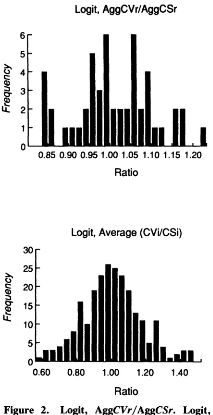
Figure 2. Logit, AggCVr/AggCSr. Logit, Average (CVj/CSi)

tically distributed Type I Extreme Value random variable, j = I for visit and j = 0 for not visit. The individual chooses to visit the site when the utility from visiting the site (V,) exceeds the utility from not visiting (Vo). The price of the activity reduces residual income (Y - Pi), for which con- stant marginal utility (B,) is assumed. Given the assumption on the error distribution, it is well known that the proba- bility of visiting (choosing j = 1) follows the logit form, with

exp(W,)

(i) prob(Visit) = ex

exp(W,) + exp(Wo) exp(B,, - By(Y - P,)) exp(Ba, - By(Y - P,)) + K

where K = exp(B,o + _By(Y - Po) If the probability of choosing to visit the site is small, then exp(W,) will be much smaller then K. Thus, the denomi- nator of (i), exp(W,) + K, can be approximated by K, so that prob(Visit) = exp(Wq)/K. Assuming (without loss of generality) that P0 equals zero, under the Poisson model with A = exp(30 + PP + /3yY), the repeat discrete choice story requires that 7r, = E[Y]/T = A/T. Equating these two probabilities, 7r, = A/T and prob(Visit) = exp(W,)/K, yields

eO+3yr+3PPP eBal+n +By(Y-PI)

In other words, the net result of the repeated discrete choice process (in terms of total visits made) can approx- imated as Poisson with A = exp(XP) = exp(00 + ByY + 0,P).'4 Moreover, the price coefficient from the count model (p,,) approximates the price responsiveness coefficient in W, (BY), and the constant term from the count model, f0, is a

reduced form incorporating Bai, T and K. Lastly, the con-

sumer surplus generated by estimating a Poisson model and using the resulting coefficients to compute the CS will be an accurate measure of the true CV.

The accuracy of the Poisson model, when a logit repeat discrete choice process is generating the data, is examined using a Monte Carlo analysis (the details of the Monte-Carlo analysis are available from the authors upon request). Briefly, a large number of individuals are created, and for each in- dividual a long (large T) repeated discrete choice process is generated. CV measures are computed, as well as the number of visits per individual. The number of visits are used in a Poisson model, and the results of the Poisson model are used to form consumer surplus estimates.

This process is repeated 50 times, with the results dis- played in figure 2. For each model, the frequencies of two ratios are displayed: aggregate CS over aggregate CV, and average CS over average CV.'5 The results clearly show that CS measures from the count model closely approximate the underlying CV (from the repeat discrete choices), with the average ratio of CV/CS quite close to 1.0.16

14 _{Note that the approximation becomes more exact as exp(W,)} + K approaches K.

"5 Aggregate CS is computed as WCSn, with the sum over all n = 1, ..., N individuals and with CSn computed at individual n's own price. Aggregate CV is computed as XCVn. Averages of an individual's CS and CV are taken over the 50 iterations.