Analysis of Different Ranges for Wireless Sensor
Node Localization using PSO and BBO and its
variants
Satvir Singh
SBS State Technical CampusFerozepur, Punjab [INDIA]
Shivangna
SBS State Technical CampusFerozepur, Punjab [INDIA]
Shelja Tayal
SBS State Technical CampusFerozepur, Punjab [INDIA]
ABSTRACT
In a Wireless Sensor Network (WSN) accurate location of target node is highly desirable as it has strong impact on overall perfor-mance of the WSN. This paper proposes the application of differ-ent migration variants of Biogeography-Based Optimization (BBO) algorithm and Particle Swarm Optimization (PSO) for distributed optimal localization of randomly deployed sensors for different ranges. Biogeography is collective learning of geographical allot-ment of biological organisms. BBO has a new inclusive vigor based on the science of biogeography and employs migration operator to share information between different habitats, i.e., problem solution. PSO models have only fast convergence but less mature. An inves-tigation on distributed iterative localization is presented in this pa-per that shows how time consumption and error varies for different ranges. Here the nodes that get localized in iteration act as anchor node. A comparison of the performance of PSO and different mi-gration variants of BBO in terms of number of nodes localized, localization accuracy and computation time is presented.
Keywords:
Particle Swarm Optimization, Biogeography Based Optimiza-tion, Enhanced BBO, Immigration Refusal, Blended BBO, Lo-calization, Wireless Sensor Networks
1. INTRODUCTION
WSN is a collection of large number of sensor nodes those are connected wirelessly in an ad-hoc manner [1]. Each node is pro-vided with sensors, transceiver, information processor and power supply, etc. The purpose of WSN is to collect and supply sensed information to a designated sink from a wider area. However, due to size, power supply and constraints the transceiving range is limited and are networked with each other to pass information to the sink. Information received at destination is of use only if the origin of the source, i.e., location of the sensor node is known. Moreover, location of all randomly deployed sensor nodes are also required to determine the route for information passing. Self organizing and fault tolerance characteristics of WSN make them promising for a number of military and civilian applica-tions [2, 3]. To determine the physical coordinates of group of sensor nodes in WSN is one of challenging problem. Some WSN challenges and constraints are Self-Management, Wireless Net-working, Design Constraints, Security.
1.1 Localization
Localization is most active research area in WSN and it usu-ally refers to the process of determining positions of unknown
nodes (target nodes) that uses information of positions of some known nodes i.e., anchor nodes based on measurements such as distance, Time of Arrival (TOA), Time Difference of Arrival (TDOA), Angle of Arrival (AOA), etc. [4, 5, 6]. Many of the applications proposed for WSN require knowledge of sensing information which gives rise to problem of localization. The lo-calization estimation is a two-phase process
involving:-(1) Ranging: Node estimates their distance from anchors (bea-cons or settled nodes) using signal propagation time or strength of received signal. Precise measurement of these parameters is not possible due to noise; therefore, results of localization algorithms that use these parameter are likely to be inaccurate.
(2) Position Estimation: It is carried out using the ranging in-formation. This is done either by solving a set of simulta-neous equations, or by using an optimization algorithm that minimizes the localization error. This is an iterative process, where settled nodes i.e., anchors and localization process is repeated until either all nodes are settled, or no more can be localized [7, 8].
2. LITERATURE SURVEY
Some Genetic Algorithms (GA) based node localization are pro-posed in [20, 21, 22, 23]. Centralized algorithm determines loca-tion of target node by estimating their distances from all one hop neighbors. Each target node is localized under imprecise mea-surement of distances from three or more neighboring anchors or settled nodes. The method proposed in this paper has follow-ing advantages over some of the earlier methods:
(1) Localization is robust against uncertainty of noise associated with distance measurement.
(2) Localization accuracy is better and has fast convergence. (3) In each iteration, one node gets settled. Thus, each node gets
more references in its transmission range. This leads to min-imization in error due to flip ambiguity, the situation that arises as reference (anchor) nodes are in non-collinear loca-tions.
This paper proposes two optimization algorithms for distributed iterative node localization in a WSN. The first algorithm is PSO [24] and second is BBO [25] and its variants, i.e., Blended BBO, Immigration Refusal, Enhanced BBO. Variants of BBO have never been proposed for distributed iterative node localization. The rest of the paper is organized as follows: Section 3 explains PSO, BBO, Blended BBO, Immigration Refusal, Enhanced BBO for localization in this study, Section 4 explains how the local-ization problem is approached using the above mentioned opti-mization methods, Section 5 discusses numerical simulation and results obtained. At the last, Section 6 presents conclusions and make a projection on possible future research path.
3. LOCALIZATION METHODS
The stochastic algorithms PSO, BBO, Blended BBO, EBBO, Refusal BBO are discussed in the following subsections.
3.1 Particle Swarm Optimization
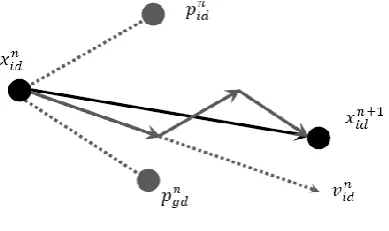
PSO is a robust stochastic optimization technique based on the movement and intelligence of swarms. It was developed in 1995 by James Kennedy (social-psychologist) and Russell Eberhart (electrical engineer). It uses a number of particles that constitute a swarm moving around in the search space looking for the best solution. Each particle keeps track of its coordinates in the so-lution space which are associated with the best soso-lution (fitness) that has achieved so far by that particle. This value is called per-sonal best ,pbest. Another best value that is tracked by the PSO is the best value obtained so far by any particle in the neighbor-hood of that particle. This value is calledgbest. The basic con-cept of PSO lies in accelerating each particle toward itspbest
[image:2.595.323.533.98.239.2]and thegbestlocations, with a random weighted acceleration at each time step as shown in Fig. 1.
Fig. 1. PSO Characterstics
Consider that the search space isM-dimensional andi-th par-ticle location in the swarm can be represented by Xi =
[xi1, xi2, ....xid..., xiM]and its velocity can be represented by
E = I
Emigration Rate () Immigration Rate ()
Mi
g
rat
ion R
at
e
HSImin HSI HSImax
Fig. 2. Migration Curves
anotherM-dimensional vectorVi= [vi1, vi2, ....vid.., viM]. Let
the best previously visited location position of this particle be denoted byPi= [pi1, pi2, ....pid.., piM], whereas,g-th particle,
i.e.,Pg = [pg1, pg2, ....pgd.., pgM], is globally best particle
lo-cation. Fig. 1 depicts the vector movement of particle element from locationxn
idtox n+1
id in(n+ 1)-th iteration that is being
governed by past best location,pn
id, global best location,p n gd,
and current velocityvn
id. Alternatively, the whole swarm is
up-dated according to the equations (1) and (2) suggested by [26], [27].
vidm+1=χ(wvidm+ψ1r1(pmid−x m
id) +ψ2r2(pmgd−x m id)) (1)
xm+1 id =x
m id+v
m+1
id (2)
Here,wis inertia weight,ψ1is cognitive learning parameter,ψ2
is social learning parameter and constriction factorχ, are strat-egy parameters of PSO algorithm, whiler1andr2 are random
numbers uniformly distributed in the range [0,1].
3.2 Biogeography-Based Optimization
BBO is a population based global optimization technique devel-oped on the basis of the science of biogeography, i.e., study of the distribution of animals and plants among different habitats over time and space.
Originally, biogeography was studied by Alfred Wallace [28] and Charles Darwin [29] mainly as descriptive study. However, in 1967, the work carried out by MacAurthur and Wilson [30] changed this view point and proposed a mathematical model for biogeography and made it feasible to predict the number of species in a habitat. For sake of simplicity, it is safe to assume a linear relationship between HSI (or population) and immigration and emigration rates and same maximum emigration and immi-gration rates, i.e.,E=Ias depicted graphically in Fig. 2. Fork-th habitat, i.e.,HSIk, values of emigration rate and
immi-gration rate are given by (3) and (4).
µk=E·
HSIk
HSImax−HSImin
(3)
λk=I·
1− HSIk
HSImax−HSImin
(4)
Algorithmic flow of BBO involves two mechanisms, i.e., migra-tion and mutamigra-tion, these are discussed in the following subsec-tions.
3.3 Migration
Migration is a probabilistic operator that improves HSI of poor habitats by sharing features from good habitats. During Migra-tion,ith habitat,Hiwhere (i= 1,2, . . . , N P) use its
[image:2.595.74.269.615.730.2]immigrate or not. In case immigration is selected, then the em-igrating habitat,Hj, is found probabilistically based on
emigra-tion rate,µjgiven by (3). The process of migration is completed
by copying values of SIVs fromHjtoHiat random chosen sites,
i.e.,Hi(SIV)←Hj(SIV). Migration variants are discussed in
the following sections:
3.3.1 Immigration Refusal. In BBO, if a habitat has high em-igration rate, i.e, the probability of emigrating to other habitats is high and the probability of immigration from other habitats is low. This BBO variants with conditional migration is termed as Immigration Refusal [31].
3.3.2 Blended Migration. In blended migration, a solution fea-ture of solutionImHbtis not simply replaced by a feature from solution EmHbt as happened in standard BBO migration op-erator. Instead, a new solution feature, ImHbt(SIV), solution is comprised of two components, i.e.,ImHbt(SIV) ← α·
ImHbt(SIV) + (1−α)·EmHbt(SIV). Whereαis a random number between 0 and 1.
3.3.3 Enhanced Biogeography Based Optimization. Standard BBO migration operator creates the duplicate solutions which decreases the diversity of the algorithm. To prevent diversity de-crease in the population, duplicate habitats are replaced with ran-domly generated habitats that increases the exploration ability.
3.4 Mutation
Mutation is another probabilistic operator that modifies the val-ues of some randomly selected SIVs of every habitat that is tended for exploration of search space for better solutions by in-creasing the biological diversity in the population. The mutation rate,mRate, fork-th habitats is calculated as (5)
mRatek=C×min(µk, λk) (5)
whereN Pis total number of habitats sorted in ascending order.
EandIare maximum emigration and immigration rates, usually
E=IandCis a constant and equal to 1.
4. STEPS FOLLOWED FOR LOCALIZATION
The objective of WSN localization is to determine maximum number ofNtarget nodes by usingManchor nodes which know their locations by the process
followed:-(1) Ntarget nodes andManchor nodes are randomly deployed in a 2-Dimensional sensor field. Each target node and anchor node has a transmission rangeR. At each iteration one node gets settled and works as anchor node in the next iteration and transmits information as the anchors do.
(2) Target node which has atleast 3 anchor nodes in its transmis-sion range is said to be localized.
(3) Mean of coordinates of anchor nodes fall within trans-mission range, i.e., mean (x1, x2, ....x5..., xn), mean
(y1, y2, ....y5..., yn)is termed as centroid position.
(4) Randomly deploy few nodes around estimated position and distance between nodes in deployment and anchor nodes in the transmission range are calculated. The distance measure-ment are effected with gaussian additive noise. A node esti-mates its distance from anchor i asdˆi=di+ηi. Wherediis
the actual distance and given by following equation
di=
p
(x−xi)2+ (y−yi)2 (6)
where(x, y)is the location of target node and (xi, yi) is
the location ofi-th anchor node in neighborhood of target node. The measurement noiseηihas a random value which
is uniformly distributed in the rangedi±di(100Pn) wherePn
is percentage noise in distance measurement.
(5) Five case studies are conducted . Each localization target node runs PSO, BBO, Blended BBO, EBBO and Immigra-tion Refusal to localize itself. The objective funcImmigra-tion is to minimize the average localization error between measured distance and estimated distance. It is defined as follows
f(x, y) = 1 M
M
X
i=1
(p(x−xi)2+ (y−yi)2−dˆi)2 (7)
whereM ≥3is the number of anchor nodes within trans-mission range R, of target node.
(6) When all theNllocalizable nodes determine their
coordi-nates, total average localization error is calculated as the mean of square of distances of estimated node coordinates (xi, yi)and the actual node coordinates(Xi, Yi), fori =
1,2,3...Nl, determines for all cases of PSO, BBO, Blended
BBO, EBBO, Immigration Refusal in following equation
El=
1 Nl
M
X
i=1
((xi−Xi)2+ (yi−Yi)2) (8)
(7) Steps 2 to 6 are repeated until all target nodes get localized. The performance of localization algorithm is based onEl
and NN l, where NN l =N -Nl is number of nodes that
could not be localized. The minimum the values ofEland
NN l, the better will be the performance.
5. SIMULATION RESULTS
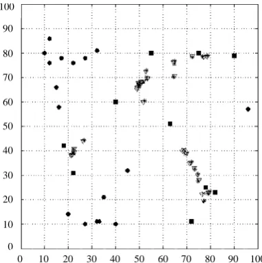
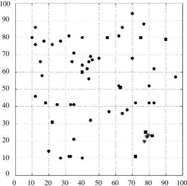
WSN localization simulations and its performance evaluation were conducted using PSO, BBO, Blended BBO, EBBO, Immi-gration Refusal in C/C++ environment. Common strategic set-tings for each case are: (1) Maximum number iterations = 20 (2) Population size = 10, (3) Number of target nodes = 50, (4) Num-ber of anchor nodes = 10 (5) Transmission range of each node = 20 and 15 respectively. These target and anchor nodes are ran-domly deployed in 2-dimensional sensor field having dimensions of100×100square units. In Fig. 3 to Fig. 12,∇defines node localization estimated by PSO, BBO, Blended BBO, EBBO and Immigration Refusal respectively,∗defines location of node,•
defines non-localized nodes and remaining defines the location of anchor nodes.
5.1 Localization using PSO
In this case study, each target node that can be localized, runs PSO algorithm to localize itself. The parameters of PSO are set as follows.
(1) Acceleration constantsc1=c2= 2.0
(2) Limits on particle position:Xmin= 0andXmax= 100
25 trial experiments of PSO-based localization are conducted for
Pn= 2andPn= 5for range20and15respectively. Average of
total localization errorEldefined in (8) is computed and shown
in Fig. 3 and Fig. 8.
5.2 Localization using BBO
In this case study, each target node that can be localized, runs BBO algorithm to localize itself. The parameters of BBO are set as follows.
(1) Limits on particle position:Xmin= 0andXmax= 100
(2) w= 0.01
25 trial experiments of localization using BBO are conducted forPn = 2andPn = 5for range20and15. Average of total
localization errorEldefined in (8) is computed and shown in
5.3 Discussions on Results
The actual locations of nodes and anchors, and the coordinates of the nodes estimated by PSO, BBO, Blended BBO, EBBO, Im-migration Refusal in a trail run are shown in Fig. 3 - Fig. 12. The best results are summarized in Table 1 and Table 2 and it can be observed that all stochastic algorithms used here have performed fairly well in WSN localization.
100
90
80
70
60
50
40
30
20
10
0 1 0 0
[image:4.595.336.522.101.290.2]0 10 20 30 40 50 60 70 80 90 100
Fig. 3. Location estimated by PSO for Range=20
100
90
80
70
60
50
40
30
20
10
0
[image:4.595.73.264.184.368.2]0 10 20 30 40 50 60 70 80 90 100
Fig. 4. Location estimated by BBO for Range=20
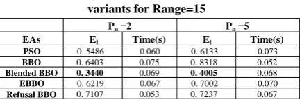
Average localization error in all algorithms is increased whenPn
is changed from 2 to 5. Performance ofElfor Blended BBO is
less as compared to all other algorithms that has been discussed. However the computing time required for Blended BBO is more as compared to BBO, EBBO, Immigration Refusal. A choice be-tween algorithms influenced by how accurate the localization is expected to be and fast convergence.
6. CONCLUSION
Artificial intelligence based single-hop distributed node localiza-tion algorithms by PSO, BBO, Blended BBO, EBBO, Immigra-tion refusal have been presented in distributed and iterative fash-ion. The proposed algorithms have better accuracy and fast con-vergence. The paper has briefly outlined the algorithms and
pre-100
90
80
70
60
50
40
30
20
10
0
[image:4.595.332.523.330.523.2]0 10 20 30 40 50 60 70 80 90 100
Fig. 5. Location estimated by Blended BBO for Range=20
100
90
80
70
60
50
40
30
20
10
0
0 10 20 30 40 50 60 70 80 90 100
Fig. 6. Location estimated by Enhanced BBO for Range=20
100
90
80
70
60
50
40
30
20
10
0 0 10
00 20 00
30 00
40 00
50 00
60 00
70 00
80 00
90 00
[image:4.595.73.263.410.605.2] [image:4.595.331.522.563.754.2]100
90
80
70
60
50
40
30
20
10
0
[image:5.595.335.523.96.286.2]0 10 20 30 40 50 60 70 80 90 100
Fig. 8. Location estimated by PSO for Range=15
100
90
80
70
60
50
40
30
20
10
0
[image:5.595.75.261.102.293.2]0 10 20 30 40 50 60 70 80 90 100
Fig. 9. Location estimated by BBO for Range=15
100
90
80
70
60
50
40
30
20
10
0
0 10 20 30 40 50 60 70 80 90 100
Fig. 10. Location estimated by Blended BBO for Range=15
100
90
80
70
60
50
40
30
20
10
0
[image:5.595.334.523.317.506.2]0 10 20 30 40 50 60 70 80 90 100
Fig. 11. Location estimated by Enhanced BBO for Range=15
100
90
80
70
60
50
40
30
20
10
0
[image:5.595.76.262.334.524.2]0 10 20 30 40 50 60 70 80 90 100
Fig. 12. Location estimated by Immigration Refusal for Range=15
sented a summary of their results for comparison. Blended BBO determines accurate coordinates quickly for both ranges20and 15but the error for range20is less as compared to range15 and time consumed is more for range20as compared to range 15. Further Stochastic algorithms can be used in centralized lo-calization method in order to compare performance of central-ized and distributed localization methods to minimize average localization error. A choice between the algorithms depends on desired localization speed and accuracy.
Table 1. Summary of 25 trial runs of PSO, BBO, and its variants for Range=20
Pn =2 Pn =5
EAs El Time(s) El Time(s)
PSO 0. 4839 0.620 0. 5777 0.618
BBO 0. 5361 0.484 0. 6692 0.547
[image:5.595.74.263.567.754.2] [image:5.595.317.542.658.741.2]Table 2. Summary of 25 trial runs of PSO, BBO, and its variants for Range=15
Pn =2 Pn =5
EAs El Time(s) El Time(s)
PSO 0. 5486 0.060 0. 6133 0.073
BBO 0. 6403 0.075 0. 8318 0.052
Blended BBO 0. 3440 0.069 0. 4005 0.068 EBBO 0. 6219 0.067 0. 7002 0.070 Refusal BBO 0. 7107 0.053 0. 7237 0.067
7. REFERENCES
[1] I. Akyildiz, W. Su, Y. Sankarasubramaniam, and E. Cayirci, “A survey on sensor networks,” vol. 40, no. 8. IEEE, 2002, pp. 102–114.
[2] D. Estrin, D. Culler, K. Pister, and G. Sukhatme, “Connect-ing the Physical World with Pervasive Networks,” vol. 1, no. 1. IEEE, 2002, pp. 59–69.
[3] G. Pottie and W. Kaiser, “Wireless integrated network sen-sors,” vol. 43, no. 5. ACM, 2000, pp. 51–58.
[4] L. Doherty, L. El Ghaoui et al., “Convex position esti-mation in wireless sensor networks,” inINFOCOM 2001. Twentieth Annual Joint Conference of the IEEE Computer and Communications Societies. Proceedings. IEEE, vol. 3. IEEE, 2001, pp. 1655–1663.
[5] R. Kulkarni, G. Venayagamoorthy, and M. Cheng, “Bio-inspired node localization in wireless sensor networks,” in Systems, Man and Cybernetics, 2009. SMC 2009. IEEE In-ternational Conference on. IEEE, 2009, pp. 205–210. [6] A. Pal, “Localization algorithms in wireless sensor
net-works: Current approaches and future challenges,” vol. 2, no. 1, 2010, pp. 45–73.
[7] G. Mao and B. Fidan, “Introduction to wireless sensor net-work localization,” 2009.
[8] N. Patwari, J. Ash, S. Kyperountas, A. Hero III, R. Moses, and N. Correal, “Locating the nodes: Cooperative localiza-tion in wireless sensor networks,” vol. 22, no. 4. IEEE, 2005, pp. 54–69.
[9] A. Boukerche, H. Oliveira, E. Nakamura, and A. Loureiro, “Localization systems for wireless sensor networks,” vol. 14, no. 6. IEEE, 2007, pp. 6–12.
[10] D. Niculescu and B. Nath, “Ad hoc positioning system (aps),” in Global Telecommunications Conference, 2001. GLOBECOM’01. IEEE, vol. 5. IEEE, 2001, pp. 2926– 2931.
[11] C. Rabaey and K. Langendoen, “Robust positioning algo-rithms for distributed ad-hoc wireless sensor networks,” in USENIX technical annual conference, 2002.
[12] A. Savvides, H. Park, and M. Srivastava, “The bits and flops of the n-hop multilateration primitive for node local-ization problems,” inProceedings of the 1st ACM interna-tional workshop on Wireless sensor networks and applica-tions. ACM, 2002, pp. 112–121.
[13] M. Di Rocco and F. Pascucci, “Sensor network localisa-tion using distributed extended kalman filter,” inAdvanced intelligent mechatronics, 2007 IEEE/ASME international conference on. IEEE, 2007, pp. 1–6.
[14] R. E. Kalman, “A New Approach to Linear Filtering and Prediction Problems,”Journal of Basic Engineering, vol. 82, no. 1, pp. 35–45, 1960.
[15] P. Biswas, T. Lian, T. Wang, and Y. Ye, “Semidefinite pro-gramming based algorithms for sensor network localiza-tion,” vol. 2, no. 2. ACM, 2006, pp. 188–220.
[16] T. Liang, T. Wang, and Y. Ye, “A gradient search method to round the semidefinite programming relaxation solution for ad hoc wireless sensor network localization,” vol. 5, 2004. [17] A. Gopakumar and L. Jacob, “Localization in wireless
sen-sor networks using particle swarm optimization,” in Wire-less, Mobile and Multimedia Networks, 2008. IET Interna-tional Conference on. IET, 2008, pp. 227–230.
[18] A. Kannan, G. Mao, and B. Vucetic, “Simulated anneal-ing based localization in wireless sensor network,” in Lo-cal Computer Networks, 2005. 30th Anniversary. The IEEE Conference on. IEEE, 2005, pp. 2–pp.
[19] A. Kumar, A. Khosla, J. Saini, and S. Singh, “Computa-tional intelligence based algorithm for node localization in wireless sensor networks,” inIntelligent Systems (IS), 2012 6th IEEE International Conference. IEEE, 2012, pp. 431– 438.
[20] G. Nan, M. Li, and J. Li, “Estimation of node localization with a real-coded genetic algorithm in wsns,” inMachine Learning and Cybernetics, 2007 International Conference on, vol. 2. IEEE, 2007, pp. 873–878.
[21] S. Yun, J. Lee, W. Chung, E. Kim, and S. Kim, “A soft computing approach to localization in wireless sensor net-works,” vol. 36, no. 4. Elsevier, 2009, pp. 7552–7561. [22] Q. Zhang, J. Wang, C. Jin, and Q. Zeng, “Localization
al-gorithm for wireless sensor network based on genetic sim-ulated annealing algorithm,” inWireless Communications, Networking and Mobile Computing, 2008. WiCOM’08. 4th International Conference on. IEEE, 2008, pp. 1–5. [23] Q. Zhang, J. Huang, J. Wang, C. Jin, J. Ye, and W. Zhang,
“A new centralized localization algorithm for wireless sensor network,” inCommunications and Networking in China, 2008. ChinaCom 2008. Third International Confer-ence on. IEEE, 2008, pp. 625–629.
[24] J. Kennedy and R. Eberhart, “Particle swarm optimization,” in Neural Networks, 1995. Proceedings., IEEE Interna-tional Conference on, vol. 4. IEEE, 1995, pp. 1942–1948. [25] D. Simon, “Biogeography-based optimization,” vol. 12,
no. 6. IEEE, 2008, pp. 702–713.
[26] X. Hu, Y. Shi, and R. Eberhart, “Recent advances in particle swarm,” in Evolutionary Computation, 2004. CEC2004. Congress on, vol. 1. IEEE, 2004, pp. 90–97.
[27] Y. del Valle, G. Venayagamoorthy, S. Mohagheghi, J. Her-nandez, and R. Harley, “Particle swarm optimization: Ba-sic concepts, variants and applications in power systems,” vol. 12, no. 2. IEEE, 2008, pp. 171–195.
[28] A. Wallace, “The geographical distribution of animals,” 1876.
[29] C. Darwin and G. Beer,The Origin of Species. Books, Incorporated, 1869.
[30] R. MacArthur and E. Wilson,The Theory of Island Bio-geography. Princeton University Press, 2001, vol. 1. [31] D. Du, D. Simon, and M. Ergezer, “Biogeography-based