http://dx.doi.org/10.4236/jamp.2015.31006
Enumeration of Strength Three Orthogonal
Arrays and Their Implementation in
Parameter Design
Julio Romero, Scott H. Murray
Faculty of Education, Science, Technology and Mathematics, University of Canberra, Canberra, Australia Email: [email protected], [email protected]
Received December 2014
Abstract
This paper describes the construction and enumeration of mixed orthogonal arrays (MOA) to produce optimal experimental designs. A MOA is a multiset whose rows are the different combina-tions of factor levels, discrete values of the variable under study, having very well defined features such as symmetry and strength three (all main interactions are taken in consideration). The ap-plied methodology blends the fields of combinatorics and group theory by applying the ideas of orbits, stabilizers and isomorphisms to array generation and enumeration. Integer linear pro-gramming was used in order to exploit the symmetry property of the arrays under study. The backtrack search algorithm was used to find suitable arrays in the underlying space of possible solutions. To test the performance of the MOAs, an engineered system was used as a case study within the stage of parameter design. The analysis showed how the MOAs were capable of meeting the fundamental engineering design axioms and principles, creating optimal experimental designs within the desired context.
Keywords
Experimental Designs, Orthogonal Arrays, Combinatorics, Parameter Design, Backtrack Search
1. Introduction
Experimental design is a well-known and broadly applied area of statistics. It started formally with the excellent book of Fisher The Design of Experiments [1] followed by the contributions of Cochran and Cox [2], Kemp-thorne [3], and complemented with the Analysis of Variance work published by Scheffe in 1959 [4].
The expansion of this field to the areas of industrial processes and engineered systems, especially through the contribution of Taguchi [5], has boosted a more detailed study of designs constructed by combinatorial tech-niques such as Hadamard matrices [6], Latin squares and their derivatives [7] [8], and orthogonal arrays of strength three [9].
among factors can be detected [10]. In order to deal with this challenge, we classified the approaches in seven categories: enumeration of the arrays, construction of algorithms, backtrack search, integer linear programming, experimental designs, parameter design, and optimality and robustness.
Techniques for enumeration of the arrays have been broadly studied through different approaches. Schoen and Nguyen [11], by using combinatorics, constructed an algorithm to enumerate a set of non-isomorphic or-thogonal arrays of given strength, run-size, number of factors and their correspondent levels. They used a tech-nique called minimum forbidden configuration. A completely different approach was developed by Schoen, Eendebak, and Nguyen [12] who enumerated pure level and mixed-level orthogonal arrays exploiting the prop-erties of asymmetric and non-asymmetric arrays based on the backtrack search algorithm.
In a similar way, two major works were undertaken using the aforementioned algorithm. Firstly, Nguyen and Murray [13] listed several designs of strength three OAs using the backtrack search technique together a C pro-gram code originally developed by Brouwer [14]. The list was initially thought to enumerate cases up to 100 runs. Secondly, a very detailed information for searching permutation and matrix groups using the backtrack al-gorithm was given by Butler [15]. He discusses the implementation of the backtrack search alal-gorithm to com-pute centralisers, intersections, and set stabilisers as well as the determinations of isomorphic groups.
Tang and Zhou [16] worked to enumerate D-optimal two-level OAs and to estimate main effects and specific interactions. This method also uses sequential collection of array’s columns and is limited to three or less two-factor interactions. Another type of enumeration and construction of OAs was published by Nguyen [9] based on the use of canonical graphs and the orbit algorithm.
Additionally to the methods previously discussed to the construction of OAs, some new approaches have seen the light. Vincent Brouerius [17] modified the C code wrote by Brouwer in order to implement parallel compu-tation to the main backtrack algorithm. Due the nature of the underlying group theory behind this implementa-tion (orbit algorithm), the results were not satisfactory. Pushing the boundaries further, He and Tang [18] intro-duced the terminology of strong OAs in terms of space filling properties. These arrays are comparable with strength three OAs but designed for computer experiments only. Moreover, Angelopoulos et al. [19] proposed an original method to the construction of OAs called step-down algorithm. This method is quite original and powerful, however is useful only for specific designs namely OA(24,7,2,t), OA(28,6,2,t), and OA(32,6,2,t), t ≥ 2. One interesting attempt of building OAs up without starting from scratch was done by Man Nguyen [20] who used Latin squares to construct strength three OAs mainly oriented to industry-based applications.
Glynn and Byatt [21] presented one of the few comparative works in constructing OAs using graphical tech-niques and projective planes. We are applying a similar technique in this research project called graph colouring developed also by Man [9]. Throughout a different perspective, Tsai, Ye, and Li [22] were able to construct a complete catalogue of geometrically non-isomorphic OAs using the Geometric Isomorphism approach. Howev-er, their enumeration was bounded to designs up to 18-runs only.
Following the idea of OAs construction, Sloane and Stufken [23] developed a linear programming bound of OAs with mixed levels, which challenges the Rao bound in order to decide the existence of some orthogonal ar-rays. Furthermore, Nguyen and Murray [24] extended the idea of orthogonal arrays construction by using integer linear programming through the algorithms provided by the mathematical software Nauty and Magma.
From the point of view of application and implementation of the orthogonal arrays, Huynh [25] showed some applications using OAs in order to solve typical experimental designs encountered in systems engineering and architecting optimisation problems. Huynh also presented the applicability of OAs to engineering testing and validation. Huynh’s work highlights one of the main features of OAs which is working directly with non-linear problems rather that their linear equivalent. In Addition, Chatzopulos et al. [26] analysed optimality criteria during the actual construction of the experimental design rather than once is already finished. Evangelaras, Ko-laiti, and Koukouvinos [27] applied the robust parameter design concept following Taguchi’s approach and embedded Hadamard Matrices. These two approaches facilitate the construction of combined arrays to over-come the product of arrays and the consequent large number of runs found in the Taguchi method. Similar work was done by Tsai [28] using the idea of a combination between combinatorial optimisation and genetic algo-rithms.
interactions calculations proposed by Byth and Gebski [31] through the use of a graphical aid. The method vi-sually helps to identify multiplicative and additive interactions effects by measuring the lost of statistical power due the presence of a particular interaction.
2. Rationale
We chose as a starting point the presentation of a case study to explain the overall idea of experimental design, and where our designs and the techniques used to construct them fit in. We also provided the theoretical back-ground to develop functional requirements (FR) and design parameters (DP) to mathematically represent the case study.
The objectives of this paper are the construction and application of experimental designs through the use of orthogonal arrays of strength three, and to make a comparative analysis against Taguchi’s technique. The study is limited to combinatorial designs and their application to the field of engineering design known as parameter design given particular attention to the design axioms and their relevance in the applicability and validity of our arrays [32] [33]. Further research makes comparative studies against traditional techniques such as cross-array designs and combined array designs [8].
3. Case Study: A Passive Filter Network
Consider the following analysis of a Passive Filter Network (adapted from [32]) which is to be designed to measure the displacement signal generated by a strain-gage transducer shown in Figure 1. This system is similar to the one used in intersections of streets to control cars’ traffic through traffic lights. The network provides the interface between the strain-gage transducer/demodulator and the recording instrument with a galvanometer/ light-beam detection indicator. The purpose is conditioning the signal generated by a strain-gage transducer with demodulated output measuring the original displacement signal by filtering out the carrier frequency [34] [35].
The functional requirements (FR) are:
• FR1 = Minimise output distortion by placing the filter pole at 6.84 Hz. • FR2 = Achieve a full-scale beam detection of ±3 in by adjusting the filter gain.
The design technique here aims to determine the correct set of descriptor parameters (DP, control factors) in order to satisfy the functional requirements. The transfer function obtained by using the Kirchhoff current law is given by:
(
)
(
)
(
)
3 0
1 2 3 3 2 3
g
g S S g S
R R V
V = R +R R +R +R R + R +R R R C (1)
where the filter cutoff frequency ωcand the galvanometer full-scale deflection D are:
(
)
(
)
(
)
2 3 3
2 3
2
g S S
c
g S
R R R R R R
R R R R C
ω
π
+ + +
=
+ (2)
(
)
(
)
0
2 3 3
| |
| |
[ ]
s S g
sen sen g S S
V R R
V D
G G R R R R R R
= =
+ + + (3)
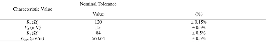
the characteristic values and tolerances for the transducer and galvanometer are shown in Table 1. Thus, the corresponding design parameters (DPs) are R2, R3, and C. Note that the values of the DPs are required to satisfy the independence axiom and the information axiom [32].
4. Description of the Approaches Applied
The aforementioned functional requirements can be achieved adjusting the characteristic values shown in Table 1. In order to find their optimal values, two approaches were used: Taguchi designs and strength three orthogon-al arrays.
4.1. First Approach: Taguchi Designs
Figure 1. A passive filter network.
Table 1. Characteristic values.
Characteristic Value
NominalTolerance
Value (%)
RS (Ω)
VS(mV)
Rg (Ω)
Gsen(µV/in)
120 15 84 563.64
± 0.15% ± 0.5% ± 0.5% ± 0.5%
quency of the filter). The selection among control factors was based on those which are both insensitive to noise factors (large η, see Equation (6)) over a broad range of values and have a linear relationship to the output re-sponse. In an ideal design, the number of DPs is equal to the number of FRs [32]. Hence, two control factors are required: one to adjust the frequency responseωc, and one to adjust the maximum light-beam deflection D. A
third condition is required, and is that the control factors (DPs) that maintain the independence of the FRs are chosen [33]. The remaining control factors (those that are not used as adjustments factors) were used to max-imise the SN ratio and minimize the information content [33].
The selection of the factor levels was made taking into consideration the broadest range of values able to yield a meaningful outcome. This is, the levels selected are representative of the range of practical possibilities [33].
Having determined the necessary combinations of the factor levels, another array (the outer array) is required for the noise factorsωc and D. This is to measure the variation in output response due the variation in the
toler-ance of the control factors. Each run yields a mean value m and a SN value η for each output response calculated according to Equations (4) and (6) [10]:
2 2
( ) ( )
E
µ
= nm −V n (4)where m is the sample mean
(
)
ny y
∑
; V is the total variation of the output y, over the entire range of n sam-ples.2 2
( ) ( m) / ( 1)
E σ = =V
∑
y −S n− (5)where ( )2
m
S =
∑
y n. The SN ratio is given by:(
2 2)
(
)
10 10
10 log E / 10 glo Sm V /nV
η
=µ σ
= − (6)and measures the variation in output due the noise factors, giving an indication of how much the desired output response changes as the tolerances of the control factors are varied over their respective ranges.
4.2. Second Approach: Orthogonal Arrays of Strength Three
{
|}
G g
g G
ω
=ω
∈ (7)In a similar way, the stabiliser is defined as [38] [39]:
{
}
( ) | g
G
Stab
ω
= g∈Gω
=ω
(8)If G acts on Ω then there is an homomorphism ϕ:G→SΩ. This is called action homomorphism [36]. By introducing the orbit algorithm, it is required the calculation of orbits and stabilisers, the representatives for each orbit, test if two arrays in
Ω
are within the same orbit (homomorphism), and store the representative arrays including the size of the automorphism group [9].Due that orthogonal arrays are actually combinatorial arrays, it is required to search for all possible permuta-tions configurapermuta-tions which satisfy certain requirements. One technique of implicitly searching all possible solu-tions in systematic manner is called backtrack search [40]. The algorithm of backtrack search enumerates the vectors (rows) starting from the lexicographically smallest, building the arrays up until either all of them are found or certain prescribed condition is violated (strength three).
In a similar way, we used canonical arrays to classify non-isomorphic fractions of a given design type and run size. This procedure encodes an array as a coloured graph to find the canonical labeling graph of the co-loured graph, and decodes the result to a fraction. Basically, the idea is to test isomorphism between coco-loured graphs rather than test isomorphism among their corresponding arrays [9].
The stages to follow for this particular approach start by translating an array to a graph assigning a specific colour to it. Then, it is required to find the canonical graph of a coloured graph; finally, the array is demerged from the coloured graph.
5. Results
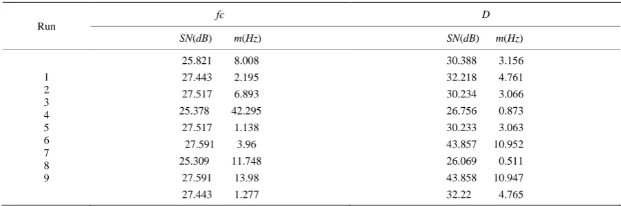
The SN ratios shown in Table 2, reproduced from [32], represent a measure of output response sensitivity to noise for the control factors’ combinations given. The sample mean m is an indication of the variation in the output response over the nine different combinations of control factor levels. These two parameters η and m, give an indication of the relative influence that each control factor has in the output response.
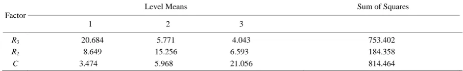
[image:5.595.86.538.468.618.2]To perform the parameter design analysis, it was also required the construction of the analysis of variance tables as shown in Table 3 and Table 4 for the SN ratio and Mean of fc respectively (reproduced from [32]).
Table 2. SN and Mean Output Responses.
Run
fc D
SN(dB) m(Hz) SN(dB) m(Hz)
1 2 3 4 5 6 7 8 9
25.821 8.008 27.443 2.195 27.517 6.893 25.378 42.295
27.517 1.138 27.591 3.96 25.309 11.748
27.591 13.98 27.443 1.277
30.388 3.156 32.218 4.761 30.234 3.066 26.756 0.873 30.233 3.063 43.857 10.952 26.069 0.511 43.858 10.947 32.22 4.765
Table 3. ANOVA for the SN ratio of fc.
Factor
Level Means Sum of Squares 1 2 3
R3
R2
C
25.503 27.517 27.517 27.001 26.755 26.781 26.927 26.781 26.829
Table 4. ANOVA for the Mean ratio of fc.
Factor
Level Means Sum of Squares
1 2 3
R3
R2
C
20.684 5.771 4.043 8.649 15.256 6.593 3.474 5.968 21.056
753.402 184.358 814.464
The passive filter network presented was worked out using the traditional parameter design technique. This method implies the calculation of one L9main factors array and 3 ×L27 noise factors arrays (a crossed design). The results for the first run were shown in Table 2, and the corresponding analyses of variance were presented in Table 3 and Table 4.
The total number of arrays needed for this design comprises 3 × 27 = 81 runs or experiments to be undertaken. Moreover, the original L27 design can handle up to 13 factors with 3 levels each (symmetric array). Hence, the selection of only 7 out of 13 columns was made arbitrarily. Moreover, although these designs are either satu-rated or near-saturated, the crossed array resulting from the product between them does not produce an eco-nomical design.
There are also some restrictions in terms of the degrees of freedom of the final crossed-design. In this situa-tion, all degrees of freedom account for main effects and control x noise interactions. No degrees of freedom account for noise x noise interactions or control x control interactions if they are required. In addition, if a new restriction needs to be checked (for instance optimality) the whole process has to be made again.
In contrast, our designs overcame these issues by meeting the design axioms of independence of functional requirements and minimization of information content. Furthermore, OA’s had the flexibility to be customised according to the factors and corresponding levels required, being economically feasible in comparison with cur-rent known techniques. The process of implementation was far simpler than its Taguchi’s counterpart, besides the feature of expandability in using more than one combination of factor levels for the same design.
There are some additional findings though that we will need to address. Firstly, we do not have knowledge about any computational technique to construct orthogonal arrays (the combinatorial form) than the method de-scribed by Hedayat [6] and the approaches proposed mainly by Schoen, Murray, and Man [11]. The former uses Hadamard matrices and the latter the orbit algorithm; both are based on backtrack search though; and secondly, we will need to undertake a comparative performance against a combined arrays design as well, which seems to be a very good competitor.
We are also considering dealing with some foreseen disadvantages and limitations of our designs, such as to choose the interactions to be measured, identify the representatives of each orbit and the size of them, choose a specific design within non-isomorphic arrays, and have enough computational power to run the algorithms.
6. Discussion and Further Studies
The outcomes of this paper and the research project can be seen in terms of two main streams: construction and enumeration of orthogonal arrays and their practical application. From the orthogonal arrays’ construction and enumeration point of view, we are working in providing a new set of isomorphism classes and sizes of auto-morphism groups for some of the incomplete designs listed in [9]. This enumeration is being performed using a special type of backtrack search algorithm. The implementation of the arrays in the context of parameter design will improve and facilitate the maintainability and reliability activities of electrical and hydraulic-powered me-chanical systems. In a similar way, using suitable comparative performance indicators, we will measure and compare pros and cons of using Crossed Array Designs, Combined Array Designs, and Symmetric Orthogonal Arrays in the context of parameter design through a new case study.
Acknowledgements
References
[1] Fisher, R.A. (1954) The Design of Experiments. Hafner Publishing Company.
[2] Cochran, W.G. and Cox, G.M. (1950) Experimental designs. Wiley Classics Library, Wiley.
[3] Kempthorne, O. (1967) The Design and Analysis of Experiments. Wiley Publications in Statistics. R. E. Krieger Pub. Co.
[4] Scheffe, H. (1959) The Analysis of Variance. A Wiley Publication in Mathematical Statistics, Wiley.
[5] Ross, P.J. (2005) Taguchi Techniques for Quality Engineering. McGraw-Hill Education (India) Pvt Limited.
[6] Hedayat, A.S., Sloane, N.J.A. and Stufken, J. (1999) Orthogonal Arrays: Theory and Applications. Springer Series in Statistics. Springer-Verlag. http://dx.doi.org/10.1007/978-1-4612-1478-6
[7] Diamond, W.J. (2001) Practical Experiment Designs: For Engineers and Scientists. Industrial Engineering/Quality Management. Wiley.
[8] Montgomery, D.C. (2012) Design and Analysis of Experiments. Design and Analysis of Experiments. Wiley. [9] Nguyen, M.M.M. (2005) Computer-Algebraic Methods for the Construction of Designs of Experiments. Technische
Universiteit Eindhoven. Eindhoven University Press.
[10] DeVor, R.E., Chang, T. and Sutherland, J.W. (2007) Statistical Quality Design and Control: Contemporary Concepts and Methods. Pearson/Prentice Hall.
[11] Schoen, E.D. and Nguyen, M.V.M. (2007) Enumeration and Classification of Orthogonal Arrays. Journal of Algebraic Statistics.
[12] Schoen, E.D., Eendebak, P.T. and Nguyen, M.V.M. (2009) Complete Enumeration of Pure Level and Mixed-Level Orthogonal Arrays. University of Antwerp.
[13] Nguyen, M.V.M. and Murray, S.H. (2007) Enumeration of Strength Three Mixed Orthogonal Arrays. School of Ma-thematics and Statistics, University of Sydney.
[14] Brouwer, A.E. (2009) A c Program Constructs 3b2a Orthogonal Arrays of Strength Three Using Depth First Search. Technische Universiteit Eindhoven.
[15] Butler, G. (1982) Computing in Permutation and Matrix Groups II: Backtrack Algorithm. American Mathematical So-ciety.
[16] Tang, B.X. and Zhou, J. (2013) D-Optimal Two-Level Orthogonal Arrays for Estimating Main Effects and Some Spe-cified Two-Factor Interactions. Metrika.
[17] Brouerius, V. (2006) Parallel Construction of Orthogonal Arrays. Technische Universiteit Eindhoven.
[18] He, Y. and Tang, B. (2013) Strong Orthogonal Arrays and Associated Latin Hypercubes for Computer Experiments. Biometrika. http://dx.doi.org/10.1093/biomet/ass065
[19] Angelopoulos, P., Evangelaras, H., Koukouvinos, C. and Lappas, E. (2006) An Effective Step-Down Algorithm for the Construction and the Identification of Non-Isomorphic Orthogonal Arrays. Springer Verlag.
[20] Nguyen, M.V.M. (2007) Some New Constructions of Strength 3 Mixed Orthogonal Arrays. Journal of Statistical Planning and Inference.
[21] Glynn, D.G. and Byatt, D. (2012) Graphs for Orthogonal Arrays and Projective Planes of Even Order. SIAM Journal on Discrete Mathematics.
[22] Tsai, K., Ye, K.Q. and Li, W. (2006) A Complete Catalog of Geometrically Non-Isomorphic 18-Run Orthogonal Ar-rays. Operations and Management Science, University of Minnesota.
[23] Sloane, N.J.A. and Stufken, J. (1996) A Linear Programming Bound for Orthogonal Arrays with Mixed Levels. Jour-nal of Statistical Planning and Inference. http://dx.doi.org/10.1016/S0378-3758(96)00025-0
[24] Nguyen, M.V.M. and Murray, S.H. (2010) Enumeration of Orthogonal Arrays Using Group Theory and Integer Linear Programming. Journal of Algebraic Statistics.
[25] Huynh, T.V. (2010) Orthogonal Array Experiment in Systems Engineering and Architecting. Department of Systems Engineering.
[26] Chatzopoulos, S., Kolyva-Machera, F. and Chatterjee, K. (2011) Optimality Results on Orthogonal Arrays Plus p Runs for s Factorial Experiments. Metrika, 73, 385-394.
[27] Evangelaras, H., Kolaiti, E. and Koukouvinos, C. (2006) Robust Parameter Design: Optimization of Combined Array Approach with Orthogonal Arrays. Journal of Statistical Planning and Inference, 136, 3698-3709.
[29] Lekivetz, R. and Tang, B. (2012) Multi-Level Orthogonal Arrays for Estimating Main Effects and Specified Interac-tions. Journal of Statistical Planning and Inference.
[30] Lekivetz, R. (2011) Optimal Factorial Designs with Robust Properties. Simon Fraser University.
[31] Byth, K. and Gebski, V. (2005) Factorial Designs: A Graphical Aid for Choosing Study Designs Accounting for Inte-raction. SCT Journal, 1, 315-325.
[32] Suh, N.P. (1990) The Principles of Design. Oxford Series on Advanced Manufacturing. Oxford University Press on Demand.
[33] Blanchard, B.S. and Fabrycky, W.W.J. (2011) Systems Engineering and Analysis. Prentice-Hall International Series in Industrial and Systems Engineering. Prentice Hall PTR.
[34] Boylestad, R. and Nashelsky, L. (2009) Electronic Devices and Circuit Theory. Pearson-/Prentice Hall.
[35] Sedra, A.S. and Smith, K.C. (1998) Circuitos Microelectronicos. The Oxford Series in Electrical and Computer Engi-neering. Oxford University Press, Incorporated.
[36] Hulpke, A. (2010) Notes on Computational Group Theory. Department of Mathematics. Colorado State University.
[37] Holt, D.F., Eick, B. and O’Brien, E.A. (2005) Handbook of Computational Group Theory. Discrete Mathematics and Its Applications. Taylor & Francis. http://dx.doi.org/10.1201/9781420035216
[38] Fraleigh, J.B. (2004) A First Course in Abstract Algebra. Addison Wesley.
[39] Artin, M. (2011) Algebra. Pearson Prentice Hall.