Finding Cost-Efficient Decision Trees

(1)

Finding Cost-Efficient Decision Trees

by

David Dufour

A thesis

presented to the University of Waterloo in fulfillment of the

thesis requirement for the degree of Master of Mathematics

in

Computer Science

Waterloo, Ontario, Canada, 2014

c

(2)

Author’s Declaration

I hereby declare that I am the sole author of this thesis. This is a true copy of the thesis, including any required final revisions, as accepted by my examiners.

(3)

Abstract

Decision trees have been a popular machine learning technique for some time. Labelled data, examples each with a vector of values in a feature space, are used to create a structure that can assign a class to unseen examples with their own vector of values. Decision trees are simple to construct, easy to understand on viewing, and have many desirable properties such as resistance to errors and noise in real world data. Decision trees can be extended to include costs associated with each test, allowing a preference over the feature space. The problem of minimizing the expected-cost of a decision tree is known to be NP-complete. As a result, most approaches to decision tree induction rely on a heuristic. This thesis extends the methods used in past research to look for decision trees with a smaller expected-cost than those found using a simple heuristic. In contrast to the past research which found smaller decision trees using exact approaches, I find that exact approaches in general do not find lower expected-cost decision trees than heuristic approaches. It is the work of this thesis to show that the success of past research on the simpler problem of minimizing decision tree size is partially dependent on the conversion of the data to binary form. This conversion uses the values of the attributes as binary tests instead of the attributes themselves when constructing the decision tree. The effect of converting data to binary form is examined in detail and across multiple measures of data to show the extent of this effect and to reiterate the effect is mostly on the number of leaves in the decision tree.

(4)

Acknowledgements

I would like to thank my supervisor, Peter van Beek and my readers Robin Cohen and Forbes Burkowski for taking the time to make this thesis better than I could have on my own.

The School of Computer Science at the University of Waterloo and all those involved in making it as successful as it is.

Christian Bessiere, Emmanuel Hebrard, and Barry O’Sullivan for their work on “Min-imising Decision Tree Size as Combinatorial Optimisation” which has inspired this thesis. Especially to Emmanuel Hebrard for providing direction.

The University of California Irvine Machine Learning Repository[3] and those who contribute to it. Special thanks to Moshe Lichman for the quick response to my request for data.

Most of all I would like to thank my friends and fellow students who were there with me through the duration of this work.

(5)

Dedication

I dedicate this thesis to my family, the people who have always been there for me and will continue to be there. Without them I would not have had the time nor inspiration to get to where I am today.

(6)

List of Tables

2.1 Dataset of patients labelled with their diagnosis. Each row represents a patient while each column represents the results of a test conducted on a patient. A question mark represents missing test results for a patient. . . . 8 3.1 Formulation of the problem of finding the smallest decision tree. The left

column contains variables related the structure of the decision tree and the data it is built from. The right column contains more information about the variables and how they are related to the decision tree. . . 28 5.1 Datasets from the UCI Machine Learning Repository used to test D4

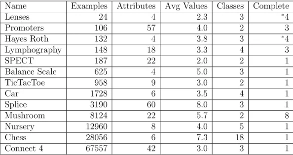
algo-rithm. The datasets are sorted by second column (the number of examples in the dataset). The third and fourth columns are the number of attributes in the dataset and the average number of values for those attributes. The second to last column contains the number of classes, while the last column is the number of top attributes that can be searched completely in under an hour. The ‘Lenses’ and ‘Hayes Roth’ datasets can look at every pos-sible decision tree with all combinations of all the attributes at all depths considered.. . . 40 5.2 Cost datasets from the UCI Machine Learning Repository used to test D4

algorithm. The columns in the table represent the number of examples, attributes, average number of values, and classes for each dataset. . . 41

(10)

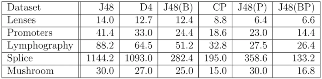
5.3 Expected costs of decision trees grown on the datasets from the UCI Machine Learning Repository. The left three columns contain information about the decision tree generated by C4.5 and the three columns on the right generated by D4. The three columns for each algorithm contain the average expected costs, sizes and generalization accuracies of the decision trees generated. The dark gray highlighted cell represents the only dataset where the D4 algorithm was able to find a decision tree of lower expected cost than C4.5. The light gray highlighted cells represent an insignficant cost reduction by D4. . . 42 5.4 Comparison between WEKA’s J48, the D4 algorithm and Bessiere et al.’s

constraint programming (CP) method on categorical data. Both D4 and CP were allowed to run for five minutes after finding it’s last solution, while J48 had no timelimit. Each cell represents the average decision tree size from each of the 10-fold cross-validation runs. . . 43 5.5 Comparison between WEKA’s J48, the D4 algorithm and Bessiere et al.’s

constraint programming (CP) method on categorical data. Each cell rep-resents the average decision tree classification accuaracy from each of the 10-fold cross-validation runs. . . 43 5.6 Comparison between WEKA’s J48 and constraint programming (CP) method

on categorical data. Average decision tree size (number of nodes) is reported for each algorithm. The ‘% of Data’ column represents the percentage of data used in the training set. The ‘WEKA’ column contains the results of J48 run on non-binary data from [5]. The ‘CP First’ and ‘CP Best’ columns contain the results of the CP method from the same paper (both the first and best decision trees found). The last two columns are original and contain WEKA’s J48 algorithm’s result when run on both binary and non-binary data. . . 46

(11)

5.7 Comparison of decision tree size between binary and non-binary features on an assortment of data. The first column on the left gives a descrip-tion of the data being used. The code 4f 4v 10e means the data has four features, four values per features and ten examples, while 2-5v specifies a range of values. The table is broken up into three sections: D4 run with no minimum number of examples required for a leaf and no pruning, D4 run with a minimum of one example required for a leaf and no pruning, and the default pruning settings of WEKA’s J48. In each of those three sections there are two columns representing the normal data as well as the data converted to have binary attributes using the method used by Bessiere et al.[5]. The three highlighted columns are to show that binary decision trees are normally smaller than their non-binary counterparts. When there is a minimum number of examples required in a leaf, binary decision trees are no longer smaller, as there are no longer empty leaves in the non-binary tree. This removes empty leaves and shrinks the size of the decision trees on data with non-binary attributes. In this experiment only the best attribute was examined as determined by the heursitc, D4 preformed no searching or backtracking. . . 49 5.8 Comparison of decision tree size between binary and non-binary features

on an assortment of data. Continuation of Table 5.7 with ten features as opposed to four. . . 50 5.10 Trends found when comparing decision tree sizes of datasets with similar

dimensions. The first column is the group that is being averaged, whether it be datasets with a hundred examples (100e), four features (4f), or eight values per feature (8v). The second column is the ratio between the size of decision trees found using the original data and the decision trees found using the data converted to have binary attributes. The third column is the ratio between the size of decision trees found using the original data with a requirement that every leaf have at least one example and the decision trees found using the data converted to have binary attributes. . . 51 5.9 Comparison of decision tree accuracy between binary and non-binary

fea-tures on an assortment of data. This table contains the training accuracies of the decision trees in Tables 5.7 and 5.8. . . 53

(12)

List of Figures

2.1 Decision tree built from Table 2.1 using the C4.5 algorithm. Patients are first tested on their response to antibiotics, with a full response immediately diagnosing patients with a bacterial infection. . . 9 4.1 Pictorial of the D4 algorithm. The left-most group of people represent

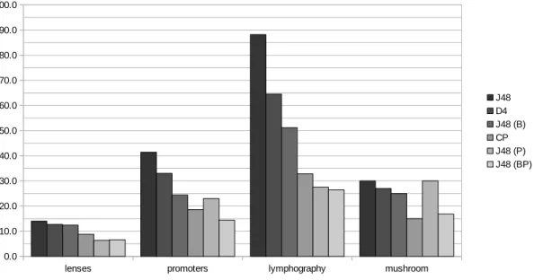
pa-tients or examples used as input into the algorithm. After being passed through the algorithm the patients are grouped by their diagnosis and or-ganized in the decision tree by the values of their tests. . . 32 5.1 Bar graph showing the average size of the decision trees generated by each

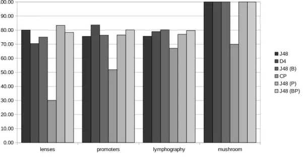
algorithm on each dataset. The Y-axis marks the average size of the ten decision trees generated by each algorithm, while the X-axis contains the datasets. Each dataset contains six bars representing the six algorithms. J48 with all pruning turned off generated the largest decision trees while J48 using binary data with pruning turned on generated the smallest decision trees. The D4 algorithm searches through many possible trees to find a smaller decision tree using multi-variate data, while the CP algorithm does the same thing but using binary data. . . 44 5.2 Bar graph showing the average accuracy of the decision trees on test data

generated by each algorithm on each dataset. The Y-axis marks the average accuracy of the ten decision trees generated by each algorithm, while the X-axis contains the datasets. Each dataset contains six bars representing the six algorithms. The CP algorithm generated decision trees with considerably lower accuracies. . . 45 5.3 Effect of converting attributes to binary. The left decision tree has

multi-valued attributes while the right decision tree has binary attributes. Notice the number of tests stays constant despite the decrease in size. . . 47

(13)

Chapter 1

Introduction

Decision trees are a simple yet powerful tool for predicting the class label of an example. There are many areas which can benefit from the use of decision trees, including image processing, medicine, and finance (these examples and more can be found in [28, p.26]). Trees are constructed from a set of training examples that share attributes and a selection of labels. These examples are recursively split into groups based on the value of the attribute being tested at a given node and sent down a branch that is associated with that value. At the end of these paths of branches are leaf nodes, or a collection of examples that all agree on what class they belong to. So when a new example is sent down the root of the tree, it will be examined by each attribute along the way, moving down the appropriate branches. At the end of a path of branches in the decision tree are similar examples in a leaf node, all sharing a classification that will be used to label the new example.

Hyafil and Rivest[18] show that the problem of finding an optimal decision tree for most measures of quality is NP-complete. Consequentially, a top down, single pass, heuristic-driven induction method is used in the construction of decision trees. Although, in practice on real world data, it might be possible to find decision trees that are smaller, or cost less than the trees found using the heuristic by searching the space of possible decision trees in a clever way. This chapter introduces the problem this thesis hopes to solve, outlines the motivation for this direction of work, states certain objectives, and summarizes the contributions of this thesis.

Generally, smaller trees are sought after when constructing decision trees. The depth of a tree can be kept small by considering the information content of the examples given a split using different attributes. The popular heuristic information gain is one way to accomplish the growth of decision trees with shorter path lengths to leaf nodes. A generalization of

(14)

the problem of finding decision trees with short paths from the root to its leaves is to add weights to the attributes at each split in the tree. Costs, risks, delays and other measures of preference over attributes can be included in the heuristic in a way that reduces the expected path length while preferring attributes at each point in the path with low costs. This creates a balancing act between the cost and accuracy of the resulting decision tree and optimizing for one doesn’t necessarily lead to the optimization of both. The solution proposed in this thesis to the problem of minimizing the expected-cost of decision tree is to iterate over a subset of viable decision trees with a bias for trees that maximize the ‘information gain over cost’ heuristic.

1.1

Motivation

In past research, C. Bessiere, E. Hebrard, and B. O’Sullivan[5] made an attempt to use constraint programming and other techniques to find the smallest decision tree consistent with some training data (classifying all training examples correctly). They reasoned that smaller decision trees were preferable for their simplicity, having relatively fewer attributes and perhaps because they would have greater generalization accuracy. Bessiere et al. found that no matter which technique they used (whether it be a SAT-solver, constraint program-ming, or linear programming), modern optimization methods could not find the smallest decision tree on anything but the smallest of datasets.

Part of the original motivation for Bessiere et al.’s work was to minimize the number of tests conducted on a patient during a diagnosis. Where they minimized the total number of internal nodes and leaves of decision trees, I look to minimize only the number of internal nodes representing tests in the tree. Of course not all tests are the same when it comes to their monetary cost, the time they take, the risk involved, etc. Imagine in the worst case, the need for an exploratory surgery on a patient. Although a decision tree that classifies all examples could be built with just one testing node (results of an exploratory surgery), the cost of that test would be very high for the patient. In between this and conducting an infinite number of zero costs tests that provide no information, we find limited resources of hospitals, wait times for biopsy and blood test results, financial burdens of different tests and many other reasons why some tests may be preferred over others. So the work of this thesis hopes to extend Bessiere et al.’s model to include a cost for each attribute used in the construction of decision trees. Although the motivation and experiments in this thesis are focused on medical examples, the methods introduced work to generalize past results on minimizing decision tree size by adding weights to each attribute and in turn minimizing the expected cost of the decision tree.

(15)

1.2

Objectives

The objective of this thesis is to extend and simplify Bessiere et al.’s model to allow for attributes and classes with more than two values and to associate costs with attributes used to split the examples of the decision tree. The goal was to find decision trees with multi-valued attributes substantially smaller than those found by a heuristic and to find decision trees with expected-cost lower than those found by a cost heuristic.

This thesis introduces and explains a new top-down breadth-first decision tree induction algorithm with backtracking and any-time behaviour (having the best solution so far ready at any-time in the algorithms runtime). The goal is to extend past optimization attempts to allow for a more general approach to minimizing different decision tree measures.

It is also the goal of this thesis to take an in-depth look at data used for constructing decision trees. More specifically, I analyse the effects of converting data to have binary valued attributes and a binary classification.

1.3

Contributions

Bessiere et al.[5] reported finding decision trees significantly smaller than those found using Ross Quinlan’s C4.5 algorithm[36] with pruning turned off. Although the D4 algorithm can find smaller decision trees, they are not nearly as small as those generated by Bessiere et al. due to them converting their data to binary. Also, in most cases the expected-cost of decision trees cannot be reduced past the expected-cost of decision trees found using the standard single pass heuristic methods. I also show that converting the attributes in data to many attributes with two values, results in smaller decision trees than the unpruned trees generated by the C4.5 algorithm. This goes against expectations when considering the straight conversion of a decision tree with multi-value attributes to a decision tree with binary value attributes, but accounts for some of the results seen in Bessiere et al.’s work. In this thesis I introduce a new algorithm that I call D4. It is a descendant of the Ross Quinlan’s ID3 algorithm[35] with some extensions that allow constraints and searching of the solution space that a simple heuristic cannot provide. It runs on categorical data with any number of attributes, values per attribute, and examples. A top-down breadth-first approach is taken when generating decision trees, with the addition of backtracking when certain bounds are passed. The D4 algorithm is highly customizable in the way it performs a search. It can generate a single decision tree equivalent to a decision tree induction algorithm that simply maximizes a heuristic or in contrast can do a complete search of

(16)

all decision trees that meet a certain criteria. Of course as the number of attributes and examples get large in a dataset, the less likely it is for a complete search to be accomplished. The D4 algorithm allows for searching a subset of the solution space as well as randomly generating decision trees with bias from a heuristic. The algorithm is an any-time algorithm and will return the best decision tree found so far when stopped. Although it cannot always find decision trees that perform better under a certain measure, the benefits from the extensibility and customizability of the algorithm make D4 a worthwhile addition to the ID3 family.

1.4

Outline of the Thesis

The remainder of this thesis will be structured as follows.

Chapter 2starts off by explaining the history of decision tree induction. Decision trees are explained in detail and measures of both size and cost of attributes are examined. Ockham’s razor as it applies to decision trees is defined and debunked as being more than a guideline for constructing accurate decision trees. Chapter 2 also discusses different heuristics used in decision tree construction, missing values in training and test data, and the pruning of decision trees.

Chapter 3is an examination of several decision tree induction algorithms. The famous depth-first ID3 and C4.5 algorithms are explained and a best-first decision tree induction algorithm is examined to contrast D4’s breadth-first approach to decision tree induction. ID3+ introduces the idea of backtracking in decision tree induction to avoid pitfalls such as insufficient examples and features during decision tree construction, which my algorithm, D4, expands on. Bessiere et al.’s work using constraint programs to optimize decision tree size is discussed and critiqued as this work is a direct extension of it. Finally, ICET, an evolutionary approach to decision tree induction is discussed for its use of attribute costs and misclassification costs.

Chapter 4discusses the D4 algorithm introduced in this thesis, while Chapter 5 evalu-ates its effectiveness. Chapter5contains other results pertaining to the search for smaller or lower cost decision trees using backtracking and randomization.

Chapter 6 closes off the thesis with remarks on what has been accomplished and an inclusion of future directions for the optimization of decision tree cost. AppendixA at the end of this thesis is included to describe a remodelling of the constraint program in [5] to work on Choco[19] and other constraint solvers. This model does not appear anywhere

(17)

else in the thesis as it does not achieve anything that has not already been accomplished, but relates to my work and can be helpful to those looking to explore this area further.

(18)

Chapter 2

Background

The background contains a brief overview of decision trees, their size, and how to construct them. It will begin by discussing the problem of finding the smallest/lowest-cost decision tree, where it is used, what the data decisions are built from look like, why it is so hard to find small decision trees, and even why we are motivated to find them.

The first section will briefly describe decision trees and the decision tree construction problem. Then Ockham’s razor will be discussed and how it relates to constructing decision trees will be explained. The popular heuristic, information gain, its use of entropy, and why heuristics are used at all will be examined. As this thesis looks to understand minimizing the expected cost of decision trees, heuristics that take cost into account will also be surveyed. Although my proposed algorithm does not take missing values into account and does not use pruning, both are important when considering decision trees and will be briefly explained at the end of this chapter.

A basic understanding of algorithms and complexity in computer science is assumed. The goal of this chapter is to give the reader an outline of the problem of finding decision trees of low expected cost and the literature surrounding that problem. Further information about decision trees can be found in the survey by Murthy[28] and information about cost-sensitive decision tree induction algorithms can be found in the survey by Lomax and Vadera[24].

(19)

2.1

Decision Trees

Decision trees have been used in machine learning for many years and their widespread use can be attributed to their ease of construction and readability. There are many application areas that decision trees are used in: some examples taken from [28, p.26] are agriculture, astronomy, financial analysis, image processing, manufacturing and production, medicine, plant diseases, and software development.

Hyafil and Rivest[18] show that constructing optimal binary decision trees, with the smallest number of expected tests to classify an example, is NP-complete. They prove com-pleteness by taking the known NP-complete problem 3DM, finding a three-dimensional matching, reducing it toEC3, the exact cover set problem where the subsets available con-tain exactly three elements, and then finally reducingEC3 to the problem of constructing an optimal binary decision tree. Their results show that finding a decision tree that clas-sifies a set of examples with the minimum number of tests is NP-complete and the result is generalizable to assigning a cost to each test. Thus, any algorithm that finds a decision tree with the lowest average expected cost of the paths in the decision tree is not going to scale well on large data sets. In these situations, a heuristic is used to find near optimal solutions.

More so, Moret[26, p.603] shows that different decision tree measures, such as tree size and expected cost, are pairwise incompatible and thus optimizing for one measure means not optimizing for the others. Approximation is also difficult. Laber and Nogueira[21] show that the binary decision tree problem does not admit ano(logn)-approximation algorithm, Adler and Heeringa[1] show this holds true for the decision tree problem with weighted tests and Cicalese et al.[9] show it holds true for the weighted average number of tests.

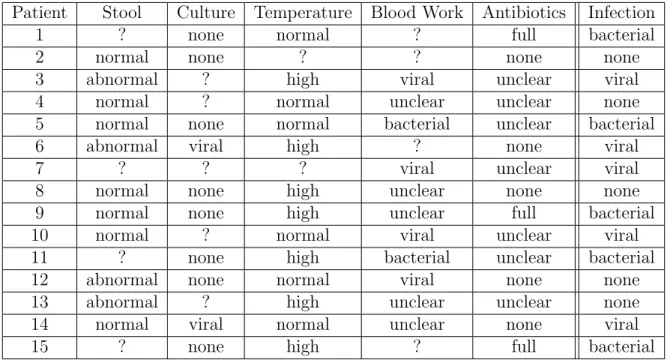
Table 2.1shows how the data for decision trees are formatted. Each row in the dataset represents an example, or specifically in the case of the infection dataset, a patient that had a series of tests conducted on them. Each column contains the results from a test and is referred to as a value of an attribute. The last column represents what class the example falls in, or again more specifically, the diagnosis of the patient. The aim of constructing a decision tree is to group patients with a similar diagnosis together by comparing the results of their tests in the hopes to later find new patients’ diagnoses.

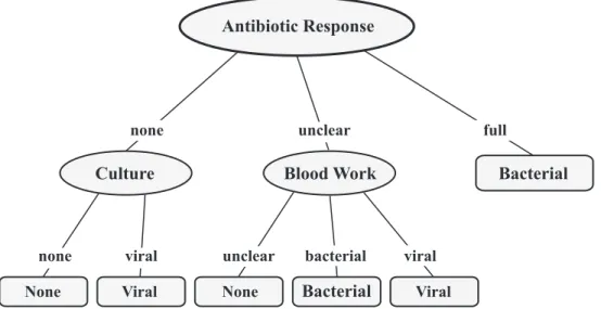
Finding similar patients is accomplished by choosing an attribute and splitting the examples into groups based on which value of the attribute or result from the test they received. Figure 2.1 shows the decision tree grown using C4.5. The ‘Antibiotics’ test is chosen for the root and the examples 2, 6, 8, 12, and 14 are sent down the leftmost branch because those patients did not respond at all to the antibiotics. Examples 1, 9, and 15

(20)

Table 2.1: Dataset of patients labelled with their diagnosis. Each row represents a patient while each column represents the results of a test conducted on a patient. A question mark represents missing test results for a patient.

Patient Stool Culture Temperature Blood Work Antibiotics Infection

1 ? none normal ? full bacterial

2 normal none ? ? none none

3 abnormal ? high viral unclear viral

4 normal ? normal unclear unclear none

5 normal none normal bacterial unclear bacterial

6 abnormal viral high ? none viral

7 ? ? ? viral unclear viral

8 normal none high unclear none none

9 normal none high unclear full bacterial

10 normal ? normal viral unclear viral

11 ? none high bacterial unclear bacterial

12 abnormal none normal viral none none

13 abnormal ? high unclear unclear none

14 normal viral normal unclear none viral

15 ? none high ? full bacterial

went down the rightmost branch because the antibiotics cleared the infection and the rest of the examples were unclear and went down the middle branch. Once the data have been split, it can be seen that the rightmost group of patients have all been diagnosed with a bacterial infection (or are all classified the same). These patients represent a leaf node in the tree that is labelled ‘Bacterial’. Any future patients’ infection cleared by antibiotics will allow for a diagnosis of a bacterial infection (or any example with the value ‘full’ for the attribute/test ‘Antibiotic’ will be classified as ‘Bacterial’). The complete tree is built by repeating the splitting process on the remaining groups of examples until all of the subgroups’ classifications are the same.

The details behind building decision trees have been left vague up until this point and the following sections will go on to explain the effects of decision tree size on accuracy, how to choose an attribute using a heuristic function, incorporating attribute costs into the model, what to do when values are missing and how to deal with noisy, missing, and erroneous data.

(21)

Antibiotic Response

Culture Blood Work Bacterial

Bacterial Viral Viral None None viral bacterial unclear unclear viral none none full

Figure 2.1: Decision tree built from Table2.1 using the C4.5 algorithm. Patients are first tested on their response to antibiotics, with a full response immediately diagnosing patients with a bacterial infection.

2.2

Data Representation: Effect on Decision Tree Size

When working with decision trees, having attributes and a classification with only two possible values makes induction easier and has some advantages that will be explained later. Real world data does not necessarily come in this form though, so a method for converting examples into binary form is required. I will discuss the two most prominent ways of converting data into binary in this section, both a direct conversion and a method that preserves the cardinality of the attribute set. Consider the following example,

@attribute stool {normal,abnormal} @attribute culture {none,viral} @attribute temperature {normal,high}

@attribute blood_work {unclear,bacterial,viral} @attribute antibiotic_response {none,unclear,full} @attribute class {none,bacterial,viral}

@data

(22)

To directly convert the example into binary form using the method used by Bessiere et al.[5], a new attribute has to be created for each value belonging to non-binary at-tributes, meaning nine attributes in place of five. For example, the attribute blood work will becomeblood work unclear,blood work bacterial, andblood work viral. So since the example has the valuebacterialfor the original attribute,blood work bacterial will be set to true while the other two are set to false. Since the class has more than two values, it will be split into two subsets. The values viral and none will be grouped together as both require no treatment. The example now has nine binary attributes and a binary class (0,0,1,0,1,0,0,0,1,1) and translates to having normal stool, no culture, high temperature, clear blood work, bacterial results from blood-work, non-viral results blood-work, an an-tibiotic response, a clear anan-tibiotic response, a full anan-tibiotic response, and is classified as a bacterial infection.

Another method for converting features into binary is proposed by Friedman et al[14]. It involves splitting the values of the attribute into subsets and finding the combination of subsets that maximizes information gain. Splitting the values of the attribute into two groups allows the size of the problem to stay the same as no new attributes are created. For the above example, there would be two attributes again that need to be made into binary attributes. The attributeantibiotic response will become the attributes antibiotic response unclearandantibiotic response f ull, which group together no antibi-otic response and an unclear response into the same attribute. The class would be grouped in a similar way as before.

Concentrating on binary classes while ignoring attributes, Polat et al.[32] propose a way to turn multi-class classification problems into binary classification problems using a one-against-all approach. The method uses C4.5 to create a decision tree for each class, labelling examples positive if they are in that class and negative otherwise. Using these decision trees together greatly improves classification accuracy over using a single decision tree that has more than two classes.

2.3

Ockham’s Razor

The most popular version of Ockham’s razor, “entities must not be multiplied beyond necessity” is a common axiom stated without reference to Ockham by John Punch[34]. The better of two equally accurate hypotheses will be simpler and make less assumptions to avoid the possibility of errors. Historically, Ockham’s razor has been used in machine learning and specifically when constructing decision trees, to justify smaller hypotheses.

(23)

This section will outline why it is important not to rely too heavily on the razor when constructing decision trees.

Ockham’s razor, named so by Sir William Hamilton in 1852 in honour of William of Ockham’s effective use of similar principles, has many interpretations. In this work, it will be taken to mean that a decision tree with fewer nodes is a simpler tree. There are clear benefits to a smaller tree as it is both easier to understand and contains fewer (possibly costly and time consuming) tests. A false interpretation of the razor would be to attribute higher classification accuracy to these “simpler” decision trees. It should be remembered that Ockham’s razor is a heuristic, not a guarantee.

The Ockham Razor bound, derived from [6], is a theoretical bound relating to Ockham’s razor. Given two hypotheses with the same error on a training set S of size m, errS(h), the upper bound on the generalization error on a testing set generated by a probability distributionD with probability greater than 1−δ,errD(h) will be higher for hypotheses, h, with a longer description length,|h|,

∀h∈ H, errD(h)≤errS(h) + r

|h|+ln(2/δ)

2m . (2.1)

The above formula may lead us to believe that decision trees with a smaller description length, or size, will always have better classification accuracy on unseen data. In general though, this is not the case and is merely a guarantee on the upper bound of the error.

Domingos[10] proposed separating the razor into two separate razors to consider when discussing knowledge discovery. The first is that simplicity should be preferred in itself and the second and false one can be stated as:

Given two models with the same training-set error, the simpler one should be preferred because it is likely to have lower generalization error[10, p.2].

Domingos[10] goes on to debunk some of the theoretical arguments for this version of the razor and to discuss the “no free lunch” theorem. Wolpert and Macready[45] state that “any two algorithms are equivalent when their performance is averaged across all possible problems.” Another way to look at it is: for every domain where a smaller decision tree has better accuracy on unseen data, there is another domain where the opposite is true. Thus, it is important to know your domain and know what you are optimizing for.

The reader may be familiar with the pruning of decision trees to avoid over-fitting and thus assume that the general goal is creating smaller trees to improve the accuracy on

(24)

unseen data. Over-fitting is when the error on training data is low, while the generalization error (error on testing data) is higher. The pruning that happens is to make sure that all the branches in the tree have statistical significance and have enough examples to justify a split or classification. Given sufficient data, there is no need to reduce the size of the tree. Although Ockham’s razor provides no theoretical guarantees that smaller decision trees always have higher accuracy on unseen data, does experimentation on real world data show that smaller trees do provide better classification accuracy on unseen data? Domingos[10] provides two sets of evidence against the idea that smaller decision trees provide higher classification accuracy. There have been experiments that contradict the relationship be-tween simplicity and accuracy, as well as the success of more complex models increasing accuracy in practice.

Murphy and Pazzani[27] investigate the relationship between the size of decision trees and their accuracy on test data. They consider decision trees with perfect accuracy on training data. Their findings show, on average, the smallest consistent decision trees are less accurate than slightly larger decision trees. However, with no prior knowledge, simpler hypotheses should be preferred as they improves accuracy when learning simple concepts and the opposite bias provides no benefit for more complex concepts.

Webb[44] examines Ockham’s razor and specifically addresses what he calls Ockham thesis, “Given a choice between two plausible classifiers that perform identically on the training set, the simpler classifier is expected to classify correctly more objects outside the training set.” This version of the razor is more general than Murphy and Pazzani’s version as it includes decision trees that are not consistent with the training data. By adding complexity to both pruned and unpruned decision trees generated by C4.5, Webb was able to increase predictive accuracy. The increased accuracy provides experimental evidence against Ockham thesis.

Needham and Dowe[29] look to support the validity of Ockham’s Razor by consider-ing message length of a hypothesis (the log probability of a hypothesis given the data) as opposed to node cardinality (or the size of the decision tree). Although the new measure for simplicity outperforms node cardinality on certain tasks, the results “did not provide undisputed evidence for Ockham’s Razor principle.” In fact, they found the shortest mes-sage lengths preformed worse than those slightly larger, despite a trend of shorter mesmes-sage lengths having lower prediction error across all the trees considered.

(25)

2.4

Heuristics

Heuristics are a way to use available data in a problem to provide guidance in finding a solution when an exhaustive search is not practical. Bessiere et al.[5] show this by finding three exact methods for finding optimal decision trees do not scale well to anything but the smallest data sets. The use of a heuristic allows an algorithm to estimate a solution or part of a solution to aid in the search for an optimal or good solution. In regard to decision trees, heuristics are used to choose which attributes should be used to structure the data. For example, the information gain heuristic uses the number of examples with certain properties to choose an attribute that reduces entropy and consequently the number of splits required to reach a leaf node[35].

Murthy[28, p.10], in work on evaluating and comparing attribute evaluation criteria, comes to the conclusion that no attribute selection rule is superior to any of the others, but the comparison of the heuristics can outline which heuristics one would use in different settings. Although the choice of heuristic can be unclear, choosing the right stopping criterion and pruning methods to avoid over-fitting is important. I found these conclusions to be true when comparing and combining the heuristics used in [2], although the similarity of the heuristics played a significant role.

The following two subsections will describe entropy and information gain, the widely popular splitting criteria that is also used in this thesis.

2.4.1

Entropy

The now famous Shannon’s entropy was popularized by Quinlan in ID3 and C4.5’s infor-mation gain heuristic. Entropy is the measure of unpredictability and the inforinfor-mation gain heuristic seeks to reduce the entropy from a set of examples by grouping them so their classifications are more in agreement.

The entropy, H, of a discrete random variable, X, with possible values x1, ..., xn and probability P(xi) is defined as,

H(X) = −X i

P(xi)log2P(xi). (2.2)

(26)

In reducing entropy, the predictability of a classification becomes higher and with no entropy it can be predicted that the group of examples represents their common classifica-tion.

2.4.2

Information Gain

To continue with the process of creating a decision tree, I have included a worked out example of calculating the information gain of an attribute. Information gain is the change in entropy from the current node to the weighted sum of the entropies of its children given the selection of a splitting attribute.

The entropy function for the infection database example is the sum of the probabilities of a certain classification/diagnosis (bacterial, viral, none) multiplied by the information content of that classification,

entropy( b b+v +n, v b+v+n, n b+v+n) =− b b+v +n log₂ b b+v+n − v b+v +n log₂ v b+v+n − n b+v +n log₂ n b+v+n .

The above equation uses b to represent the number of examples classified as bacterial infections, v as the number of examples classified as viral infections and n as examples classified as no infection.

Information gain calculates the entropy of the examples after the split on some attribute and subtracts it from the entropy of the examples at the node you are splitting. In this example, |Eb

i| is the number of examples in node i classified as bacterial and |Ei| is the number of all of the examples associated with node i. The set Vk contains the values for attribute k. The set Ej ⊂ Ei is all of the examples in Ei that have value vj ∈ Vk when tested on attribute k. The information gain is then given by,

IG(nodei, attributek) = entropy( |Eb i| |Ei| ,|E v i| |Ei| ,|E n i | |Ei| )− X vj∈Vk |Ej| |Ei| entropy(|E b j| |Ej| ,|E v j| |Ej| ,|E n j| |Ej| ). (2.3)

(27)

Starting at the top of the decision tree for the infection dataset, there are 15 examples with 5 of each of the classifications. The attribute chosen for this example is the one with the highest information gain, antibiotic response. There are 5 examples that have no response, 3 examples with a full response and 7 examples with an unclear result. For each of the three values of antibiotic response, the examples are again split up into their classification to calculate entropy for the examples with each value,

IG(root, Antibiotics) = entropy( 5 15, 5 15, 5 15)− 5 15entropy( 0 5, 2 5, 3 5) − 3 15entropy( 3 3, 0 3, 0 3) − 7 15entropy( 2 7, 3 7, 2 7) = 1.5−0.333×(0 + 0.529 + 0.442) −0.200×(0 + 0 + 0) −0.467×(0.516 + 0.524 + 0.516) = 0.535.

The calculation of each attribute’s information gain is done every time an attribute needs to be selected for splitting the examples up and the one with the highest information gain is chosen. An attribute unused by an ancestor node will have to be selected each time the data is recursively split until the examples at each leaf node can be used to confidently label them with a classification.

2.4.3

Cost Heuristics

The original goal of this thesis was to extend the constraint programming method to minimize the size of decision trees proposed by Bessiere et al.[5] to include a cost for each attribute. The reasoning behind extending their method of searching for decision trees using a tree size heuristic is that not all tests are created equal. If the data for an example to be classified need to be collected in some way, finding the value of an attribute could take time, cost resources, or have a significant risk associated with it. The task of minimizing the size of a decision tree without taking into consideration the cost of the tree is incomplete in domains such as health care. Although this thesis only concentrates on the cost of a test, there are many other ways to include costs when building decision trees[43].

(28)

There has been some work done on adding costs to attributes in the past, through the inclusion of costs into the greedy search function in some way[30][31][41]. There has also been work done to minimize the cost incurred from misclassification and some work that does both in a way similar to my approach[42]. These are discussed further in Chapter 3.

The cost heuristics considered when designing my algorithm are adopted from Turney’s[42] cost-sensitive classification of decision trees. This section looks at the heuristics used in cost-sensitive decision tree construction algorithms IDX, CS-ID3, EG2, and ICET. All of the heuristics share the ratio of information gain over cost and thus share similar perfor-mance when minimizing cost measures of decision trees.

The cost heuristic used in Norton’s algorithm IDX[30] which was inspired by GOTA[16] considers both change in information gain (∆Ii) and the cost (Ci) of adding the next branch level i,

∆Ii Ci

. (2.4)

No justification for this ratio is given beyond the past successes of information gain in reducing the height of a decision (the length of the path to a leaf node) combined with the fact that we wish to reduce the expected cost.

Cost-Sensitive ID3[41] (CSID3) modifies Nez’s heuristic used in EG2[31] without any justification and ends up with the heuristic,

∆Ii2 Ci

. (2.5)

I chose to use the heuristic used in CSID3 in my experiments as none of the heuristics performed better than any other[42] and it contained no parameter to adjust.

The information cost function (ICF) considers a cost/benefit approach to designing the heuristic[31]. Nez also includes the parameter 0 ≤ ω ≤ 1 to allow the user to calibrate the factor of economy, or how much cost is taken into consideration when choosing an attribute,

ICFi =

2∆Ii −₁ (Ci+ 1)ω

. (2.6)

There is no information on how to set the parameterω. Turney[42] uses the heuristic from EG2 in ICET (with the ω parameter set to 1) to allow for greater control over the cost bias, although he claims that there is no reason to choose one heuristic over another.

(29)

2.5

Missing Values

A lot of real world data is not complete or error free. There is a strong possibility of encountering missing values for the attributes of training examples and any future examples we hope to classify. There are many approaches to dealing with missing values and some of those will be discussed below. Information about dealing with missing values in data that have attribute costs and misclassification can be found in [23], [22], and [47]. Although I am discussing missing values in the background, my work does not handle or deal with missing values in any way.

When building a classifier, the easiest route would be to completely ignore any exam-ples that have missing values in them. However, if the number of training examexam-ples is limited and a high percentage of the data is missing, doing so would be wasting informa-tion. Another approach is to only ignore examples with a specific attribute missing in the calculations for the heuristic of that same attribute. This still wastes information and an alternate approach can be found in Quinlan’s C4.5[36]. Quinlan handles missing values for attributes by sending each example down every branch with a weight attached to it. If the value is known, then that weight is 1 for its corresponding branch, while the weight is 0 for all other branches. Otherwise, the weight of an example for a given value’s branch is the frequency of that value in the examples at the current node. When encountering a missing value for an attribute in an example to be classified, the example is similarly split and weighted according the the probabilities of each possible value.

It is possible that the reason for missing data is the same across all of the examples collected for training. In this situation, missing data is actually information and can be taken advantage of when building decision trees. One way to do this is to add an additional branch to associate with examples that have missing values for an attribute. That way, when future examples with a missing value for an attribute need to be classified and are tested on that attribute, they can be sent down the branch associated with missing values. A similar approach could be to hold examples with a missing value for an attribute at the node where the attribute is tested. This node would be treated as a leaf node when an example to be classified is missing a value for that attribute.

A classification centric design for dealing with missing values builds a decision tree for each unclassified example. If the example has a missing value for an attribute, that attribute is not considered in the construction of the decision tree. This problem relates to the problem of selecting subsets of attributes to learn on and would be used in conjunction with other approaches for building a decision tree when values are missing in the training data.

(30)

Lastly, it is also possible to use imputation to replace missing values in the data with a value chosen using statistics about the data. This could be as simple as choosing the average value among the examples or the average value among the examples with the same classification. It can also be much more complicated and use a statistical method or machine learning itself to impute the missing values. For example, setting the attribute with missing values as the class and using the examples with known values, will allow C4.5 to classify the missing values in the data.

2.6

Pruning

A common way to improve the generalization accuracy of decision trees is to prune off sub-trees and replace them with leaves. To avoid over-fitting (the problem of matching the training data while losing accuracy on test data) it is important to have enough data to support a classification. Pruning sacrifices accuracy on training data by combining examples in multiples leaves into one leaf in the hopes of improving accuracy on unseen data. There are two main types of pruning, pre-pruning and post-pruning. Pre-pruning stops the growth of trees when splitting the data is no longer beneficial and results in decision trees that are not consistent with the training data. Post-pruning is done after a consistent decision tree is grown and uses a subset of the training data that was set aside to determine where to prune in the decision tree.

A difficulty with real world data is that it can contain noise that our learners would use in the construction of the model. The idea of pruning was proposed by Breiman[8] as an alternative to stopping the growth of a decision tree. Pruning is the act of revisiting a decision tree after it is constructed and removing sections of the tree that are not supported by the data or contributing to the classification accuracy of the tree. Otherwise trees can become too large and over-fit the data. This means that errors and noise have been used in the construction of the decision tree and the accuracy of the decision tree on unseen data will suffer. The reader is directed towards [36],[28],[24],[25],[8],[7], and [12] for more information about specific pruning methods1_.

2.7

Summary

In this chapter I covered the background for this thesis, namely decision trees and research related to constructing them. I discussed what decision trees are, how they are created

(31)

and the hard problem of finding an optimal decision tree. I also looked at Ockham’s razor and how it relates to the decision tree problem. Heuristics, including cost heuristics, were discussed as they are a necessary component when building small, low-cost decision trees. I also briefly looked at missing values in data and what pruning is and how it can improve decision trees.

In the next chapter I will discuss research related to my thesis, including the C4.5 algorithm which I compare my approach against as well as a constraint programming approach that I re-evaluate in Chapter5.

(32)

Chapter 3

Related Work

This chapter covers a few algorithms to give a historical sense of the D4 algorithm intro-duced in this thesis, it covers different decision tree construction strategies related to depth, breadth, and best first growth of decision trees and describes the algorithms extended by D4 and that I compared D4 against to determine its performance.

The D4 algorithm is a successor to the ID3 algorithm as it does not include the exten-sions made in the C4.5 algorithm, although extenexten-sions of my own are made. In Chapter5, I evaluate D4 on data with attributes that have costs and use C4.5 to create a simple deci-sion tree using the same cost heuristic used in D4. The ID3+ algorithm, another extendeci-sion to ID3, introduces the idea of backtracking to resolve issues seen in the construction of decision trees, such as running out of attributes or examples as the tree is grown. I found this idea useful and extended the use of backtracking to include upper-bounds on decision tree size and cost. I also discuss a constraint programming approach that works on binary data, as the results of the approach will be re-evaluated later in this thesis.

3.1

ID3

In 1986, Ross Quinlan introduced ID3, a way to inductively build decision trees[35]. ID3 belongs to a family of learning systems called ‘Top-Down Induction of Decision Trees’, where a tree is built recursively by splitting up data and sending subsets of the data down branches until some stopping condition is met. Quinlan recognized that the generation of all decision trees for a data set would only be possible for small induction tasks and designed ID3 to build a single, although not optimal, tree from a subset of the available

(33)

data. If the decision tree does not classify all of the training data correctly, a subset of the incorrectly classified data is added to the original subset and ID3 is run again. Algorithm 1 presented below uses information gain to choose which attribute to use when splitting the data.

Algorithm 1 Quinlan’s ID3

Let E be all training examples, A be the attribute

while Decision tree made with E0 ⊂E does not classify E do Randomly select subset of examples, E00 where E0 ⊂E00 E0 ←E00

ID3(E0,A) end while

function _ID3(E0, A)

if e∈E0 belong to the same class then return a leaf node labelled with this class end if

if A=∅then

return a leaf node with the most common class as label end if

a ←a0 ∈A that maximizesgain(a0) for vi ∈a do

LetE_i0 ⊂E0 with value vi ∈a if E_i0 =∅ then

create a leaf node with the most common class as label else

ID3(E_i0, A− {a}) end if

end for end function

The following equation for entropy is the same as Shannon’s entropy (equation 2.2) seen in Chapter 2. The number of positively classified examples, p, and the number of negatively classified examples, n, are used to find the probabilities used in the entropy calculation. It is used in ID3’s information gain calculation as an impurity measure,

I(p, n) = − p p+nlog2 p p+n − n p+nlog2 n p+n. (3.1)

(34)

The equation for E(A) is a weighted sum of the entropies of the possible values, value 1 to valuev, an attribute can have,

E(A) = v X i=1 pi+ni p+n I(pi, ni). (3.2)

Below is the classic information gain heuristic seen in ID3, C4.5 and many other decision tree induction algorithms,

gain(A) = I(p, n)−E(A). (3.3) It is noted in the original paper that I(p, n) is redundant as it stays constant for all attributes. The same results can be obtained by minimizing E(A).

A problem with the gain criterion is that it favours attributes with more values. Imagine an attribute called “label” that had a unique value for each example in the data set. This attribute would be chosen at the root using the gain criterion because the information gain would be maximized as all of the branches would contain exactly one example (one classification). This is obviously not helpful as the labelling of the data was arbitrary and provides no information. A solution to the problem proposed in Quinlan’s paper is to include the intrinsic value(IV) of an attribute,A, in the selection criteria,

IV(A) = − v X i=1 pi+ni p+n log2 pi +ni p+n . (3.4)

This allows the number of values that an attribute has to be used in the new ‘gain ratio criterion’. This ratio takes the attributes with above average gain and finds the attribute that maximizes the following,

gainratio(A) = gain(A)/IV(A). (3.5)

Although ID3 is simple, the spirit of the algorithm lives on in most decision tree in-duction algorithms to this date. The D4 algorithm introduced in this thesis is a direct descendant of ID3 with the inclusion of backtracking and costs for attributes.

(35)

3.2

C4.5

C4.5 is Quinlan’s extension of his original ID3 algorithm[36]. It has the same basic structure as ID3:

1. Run through examples and check for stopping criteria.

2. For each attribute available, calculate information gain/gain ratio.

3. Chose the attribute with highest gain and split examples across groups based on their values. Each value will correspond to a branch that leads to another node with either an attribute to split the new subset of examples or a leaf node with a classification of the examples.

4. Recursively build the sub-trees from the child nodes’ examples.

Although the structure is the same, C4.5 is able to handle missing values and continuous attributes, and has pruning and stopping criteria built in.

Missing values in an example are handled by ignoring those examples in gain calcula-tions for the attribute whose value is missing. For the classification of an example with missing values, the example is split at any nodes with attributes for which the example is missing values, into probabilities based on the fraction of examples int the node. For ex-ample, if there is no value for culture on an unseen exex-ample, the example will be classified as 0.25 viral, 0.75 none as there is one example in the viral leaf and three examples in the none leaf.

Continuous or numeric attributes are handled by creating an attribute associated with a binary split of the values for each attribute in the data set. This groups all of the examples into two parts for the gain calculation, all examples with values less than a particular example are considered to have the same value in the new binary attribute and all examples with values greater than or equal to that example are the other value. The split in the examples with the highest gain is chosen and the examples are passed down two branches.

C4.5 allows the user to specify how many examples are needed to create a leaf node. This prevents classification of unseen data without any data to support that classification. C4.5 also uses all of the training examples to create confidence intervals for post pruning where depending on these error estimates, sub-trees are replaced by leaves or their own sub-trees. This is known as sub-tree replacement and sub-tree raising.

(36)

In the results section of this thesis, C4.5 is extended to use the heuristic from Cost-Sensitive ID3 seen in Chapter2 in place of the information gain heuristic and to acts as a baseline of performance when finding decision trees of low cost.

3.3

ID3+

Xu, Wang, and Chen’s[46], Improved Decision Tree Algorithm: ID3+ _{(see algorithm} _2),

hopes to improve on the ID3 algorithm by including backtracking. They claim that ID3’s information gain heuristic favours decision trees with short path lengths from root to leaf as opposed to correct decision trees that have at least one supporting example in each leaf. Instead of stopping the growth of the tree when the branch runs out of available examples or features, ID3+ will backtrack up the tree and choose the next best feature given some heuristic. This allows their algorithm to search the solution space for a tree that classifies the data perfectly and with enough data in each leaf to support the classification.

Through their experimental results, Xu et al. show that they can find decision trees that more accurately fit the training data on two of the four data sets that were not classified with 100% accuracy by ID3. Although the idea of backtracking is useful, their algorithm can result in no tree being found if there isn’t a decision tree consistent with the data.

3.4

Best-first Decision Tree

Friedman et al.[14] introduce the idea of a best-first expansion of decision tree nodes in their work on boosting as seen in algorithm 3. The strategy of stopping growth early to save computation works best when you expand the nodes that have the best information gain first, leaving nodes with less potential to reduce entropy unexpanded. Growth can be stopped after a certain size, amount of time, or entropy has been reached.

Shi[40] proposed a best-first expansion of decision tree nodes, which has certain ad-vantages despite generating the same tree that a depth-first expansion will generate. By expanding nodes in best-first order, pruning can be approached differently. In contrast, depth-first expansion is the simplest expansion with the least overhead and breadth-first expansion is useful for backtracking and making decisions at each layer of the decision tree. As with most decision tree induction on real world data, after a certain number of expansions and as the tree grows, it will become less accurate. To deal with over-fitting, Shi uses both pre-pruning and post-pruning to contain the size of the decision tree.

(37)

Algorithm 2 ID3+

Let E contain the examples and A contain the attributes function _ID3+_(E, _A)

if alle∈E are classified the same then return a leaf node with this classification end if

if A is empty or E is empty then return NIL

end if

while A 6=∅ do

a←− next best attribute fromA for all value vi ina do

Let Ei be the subset of examples with vi if ID3+(Ei,A\ {a}) =N IL then

destroy sub-tree goto while end if

end for

return an internal node with children from ID3+

end while return NIL end function

(38)

Algorithm 3 Best-First Decision Tree

LetA be a set of attributes,

LetE be the training instances,

LetN be the number of expansions,

LetM be the minimal number of instances at a terminal node

function BFTree(A, E, N, M)

if E=∅ then return failure end if

Calculate the reduction of impurity for each attribute in A on E at the root node RN

Find the best attribute Ab ∈A

Initialise an empty listN L to store nodes

Add RN (with E and Ab) intoN L

expandTree(N L, N, M)

return a tree with the root RN; end function

function expandTree(N L, N, M)

if N L=∅then return ; end if

Get the first node FN from NL;

Retrieve training instances E and the best splitting attribute Ab of FN; if E=∅ then

return failure end if

if the reduction of impurity ofF N = 0 or N is reachedthen

Make all nodes in N Linto terminal nodes

return end if

if the split of F N onAb would result in a successor node with less thanM instancesthen

MakeF N into the terminal node

Remove F N fromN L

expandTree(N L, N, M) end if

Let SN1 and SN2 be the successor nodes generated by splitting F N on Ab on E

Increment the number of expansions by one;

Let E1 and E2 be the subsets of instances corresponding toSN1 andSN2;

Find the corresponding best attributes Ab1 forSN1;

Find the corresponding best attributes Ab2 forSN2;

PutSN1(withE1andAb1) andSN2(withE2 andAb2) intoN Laccording to the reduction

of impurity;

(39)

Best-first pre-pruning stops the expansion of the trees when the error estimates increase with further splitting. The size of these trees is used as a stopping criteria for the final decision tree. Like all pre-pruning, Shi’s method has the potential to stop too soon. Best-first post-pruning solves this problem at the cost of additional computation time.

3.5

Constraint Programming Approach

Constraint programming[38] is a programming paradigm used to solve combinatorial prob-lems where a user declares a problem and specifies constraints for a constraint solver. These constraints limit the values a variable can take on within its domain based on relationships between the variables. A constraint solver assigns values to the variables as it searches for a solution, shrinking the available values for a variable by constraint propagation and backtracking to variable assignments that agree with the constraints.

Bessiere, Hebrard, and O’Sullivan[5] use constraint programming to attempt to solve the smallest decision tree problem. Most approaches to decision tree learning use greedy algorithms and heuristics to grow a single tree from the data, while Bessiere et al. take the principle of Ockham’s razor to the extreme and look to systematically search the space of consistent decision trees for the smallest. An example presented for the motivation of finding the smallest decision tree is to reduce the number of tests in a diagnosis.

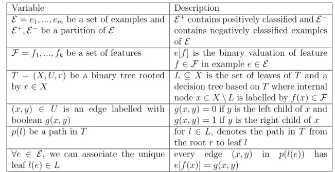
They formulate the problem of finding the smallest decision tree that is consistent with a set of training examples as follows in Table 3.1.

A decision tree classifies a set of examples E if and only if ∀(ei ∈ E+, ej ∈ E−), l(ei)6= l(ej) (no two examples in a leaf have different classifications). So, given a set of examples E, the goal is to find a decision tree that classifies E with a minimum number of nodes.

To solve the smallest decision tree problem, Bessiere et al. propose using a constraint programming model. They set an upper bound (initially found using the information gain heuristic) on the size of the decision tree and search for a binary tree with nodes less than or equal to the bound. Most of the variables in the constraint program pertain to the relationship between the nodes and defines the structure of the tree. This is unnecessary overhead as the structure of the decision tree is implied in it’s top-down induction and can be reduced to just the variables concerning the feature and examples associated with a node. As well, the majority of the constraints are associated with the structure of the tree. This is unnecessary as they find that this model does not scale well enough to explore any significant portion of the search space. To solve this problem, they subvert any gains their approach may have by employing the information gain heuristic seen in

(40)

Table 3.1: Formulation of the problem of finding the smallest decision tree. The left column contains variables related the structure of the decision tree and the data it is built from. The right column contains more information about the variables and how they are related to the decision tree.

Variable Description

E =e1, ..., em be a set of examples and E+_,_E−

be a partition of E

E+_{contains positively classified and}_E− contains negatively classified examples of E

F =f1, ..., fk be a set of features e[f] is the binary valuation of feature f ∈ F in example e∈ E

T = (X, U, r) be a binary tree rooted byr ∈X

L ⊆ X is the set of leaves of T and a decision tree based onT where internal nodex∈X\L is labelled byf(x)∈ F (x, y) ∈ U is an edge labelled with

booleang(x, y)

g(x, y) = 0 ifyis the left child ofxand g(x, y) = 1 if y is the right child of x p(l) be a path in T for l ∈ L, denotes the path in T from

the root r to leaf l ∀e ∈ E, we can associate the unique

leaf l(e)∈L

every edge (x, y) in p(l(e)) has e[f(x)] = g(x, y)

C4.5 to construct the tree top down. Essentially running the C4.5 algorithm multiple times through backtracking, the authors found that this itself is even too slow and must constrain the available features to just the features with top three information gain values at each node. It should be noted that limiting the available features to the top three features when constructing the decision tree is NP-complete.

DECISION-TREE. Given a set S of n points in R3, divided into two concept classes ‘red’ and ‘blue’, is there a decision tree T with at most k nodes that separates the red points from the blue points?

Theorem: DECISION-TREE is NP-complete[15]

This search method, coupled with a restart strategy, makes it appear as though signif-icantly smaller decision trees are found. In Chapter 5, this thesis claims that the size of the decision tree approaches that of the decision tree found using C4.5 and only after that are some gains made. Their experimental results show that the first decision trees they find are significantly smaller than unpruned decision trees found by C4.5. How can this

(41)

be when their algorithm does not look to maximize the same heuristic employed by C4.5? This can be explained by the conversion of the data to have binary attributes to allow it to be used in their model. They do not convert the data when passing it to C4.5 and thus it generates larger decision trees containing empty leaves. It then comes as no surprise that the pruned decision trees created by C4.5 are almost always smaller than the best decision trees found by the constraint program. There are no empty leaves and C4.5 always chooses the feature that maximizes information gain, instead of mucking around with lesser feature choices. Chapter 5, containing the results of this thesis, goes into greater detail on the effect that converting the data to contain binary attributes has on the problem, as well as showing some of the results of Bessiere et al. can be obtained merely by passing the binary data to C4.5.

3.6

ICET

Turney [42] looks at dealing with two types of costs when building decision trees, both costs associated with attributes and the cost of classification errors. The task of minimizing the cost of the decision tree is accomplished by employing genetic programming, an algorithm that evolves a population of biases for the decision trees generated by a modified C4.5. Turney is motivated in the same way as Bessiere et al., in that medical diagnosis requires tests, although Turney also deals with the fact that these tests have varying costs and costs associated with classification errors.

Turney’s algorithm for cost-sensitive classification, called ICET (Inexpensive Classi-fication with Expensive Tests) uses a modified version of C4.5 which includes costs. It evaluates the fitness of a bias by the classification cost of the decision tree it grows com-bined with the cost of classification errors. The biases undergoing evolution contain the costs used in the generation of the decision tree, a parameter for controlling the sensitivity to cost, and a parameter to control the level of pruning used in C4.5.

Turney’s experiments show that ICET outperforms basic heuristic single growth algo-rithms when minimizing cost. It is unclear though if their results are due to a superior algorithm or if the difference in decision tree cost between C4.5 using EG2 and ICET (which uses EG2 as its heuristic) is caused by C4.5 with EG2 not optimizing at all for mis-classification cost and thus missing out on half of the available information. Unfortunately, they do not test the performance of ICET when only considering attribute costs and thus it is not known whether or not they can reduce the average cost of a decision tree where D4 cannot. It would be interesting to see if an algorithm that took both kinds of costs

(42)

into consideration as well as performing a more straight-forward search of the decision tree space would be competitive with ICET in both speed and performance.

3.7

Summary

In this section I discussed several methods for constructing decision trees: traditional heuristic based methods such as ID3 and C4.5 as well as more modern approaches that use backtracking and different forms of search to optimize a decision tree in size or cost. Overall I looked at different methods of decision tree induction to give a sense of where the D4 algorithm I introduce fits in.

In the next chapter, I will introduce and explain my proposed method for solving the problem of minimizing the expected cost of decision trees.

(43)

Chapter 4

Proposed Method

In this chapter I introduce the D4 algorithm, a supervised machine learning algorithm. The input it takes is a set of labelled examples, such as the data in Table2.1. Following the running example, the input to the algorithm would be a set of patients who have already been diagnosed as having a viral, bacterial or no infection based on some tests that were run on the patients. What D4 outputs is a decision tree, a grouping of patients with the same diagnosis and similar test results. The decision tree is used to diagnose future patients, using their tests results to find similar patients and assign a classification. Figure 4.1 gives a pictorial of the process.

The decision tree is computed layer by layer until the cost of the decision tree becomes too high and new combinations are tried at previous layers. The process begins at a root node containing all of the examples and the attributes available with which to split the examples with. Similar examples are sent down each branch to repeat the process until all of the examples have the same classification. If at any point the size, cost or other measure of the decision tree surpasses the running upper-bound(starting off with the decision tree found using a heuristic), the examples are regrouped up to a point and subsequently split down new branches using different attributes. This can be done randomly or exhaustively until all decision trees are considered. After